Dot Plots in R

The “dot plots in R” typically refers to two distinct types of visualizations: (i) Cleveland dot plots (for comparing categories) and (ii) Stacked (Wilkinson) dot plots (for showing distributions). A dot plot is a graphical representation that breaks the range of data into many small equal-width intervals and counts the number of observations in each interval. The interval count is superimposed on the number line at the interval midpoint as a series of dots (stacked if repeated), usually one for each observation. For $mpg$ from the $mtcars$ dataset, the intervals are centered at integer values, so the display gives the number of observations at each distinct observed head breadth.

Dot Plots in R Language using Base and ggplot2 Packages

Plotting Dot Plot using R Base Graphics

The following code may be used to draw a dot plot using R Base Graphics

attach(mtcars)
par(mfrow = c(3, 1))
# Dot Plot 1
stripchart(mpg, main = "Miles per Gallon", xlab = "mpg")

# Dot Plot 2
stripchart(mpg, method = "stack", cex = 2, 
           main = "Miles Per Gallon (with Stack Method)")

# Dot Plot 3
stripchart(mpg, method = "jitter", cex = 2, frame.plot = FALSE, 
           main = "Mile Per Gallon (with no frame & Jitter Method")
Dot Plot Using R Base Package

Plotting a Dot Plot using the ggplot Package

The following code may be used to draw dot plots in R using the ggplot2 package:

library(ggplot2)
library(gridExtra)

# Dot Plot 1
p1 <- ggplot(mpg, aes(x = mpg))
p1 <- p1 + geom_dotplot(binwidth = 2)
p1 <- p1 + labs(title = "Miles per Gallon")
p1 <- p1 + xlab("MPG")

# Dot Plot 2
p2 <- ggplot(mpg, aes(x = mpg))
p2 <- p2 + geom_dotplot(binwidth = 2, stackdir = "center")
p2 <- p2 + labs(title = "Miles per Gallon (stackdire = center")
p2 <- p2 + xlab("MPG")

# Dot Plot 3
p3 <- ggplot(mpg, aex(x = mpg))
p3 <- p3 + geom_dotplot(binwidth = 2, stackdir = "centerwhole")
p3 <- p3 + labs(title = "Miles per Gallon (stackdir = centerwhole)")
p3 <- p3 + xlab("MPG")

grid.arrange(grobs = list(p1, p2, p3), ncol =1)
dot plots in R using ggplot2 package

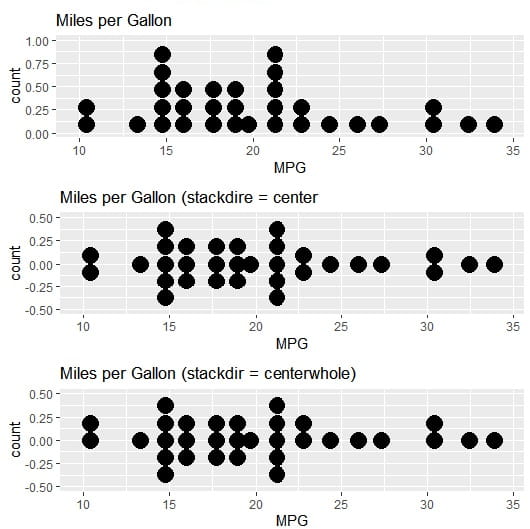
Adjust Binwidth: You can manually set the binwidth parameter to change the size of the bins the dots fall into. This helps adjust the granularity of the visualization.

Dot Plots in R Group by a Categorical Variable

One can use a categorical variable, such as cyl (number of cylinders), to group the dots and display the distribution for each group. The cyl variable needs to be converted to a factor first for proper display. The code is

ggplot(mtcars, aes(x = mpg, fill = factor(cyl))) + # Map 'cyl' to fill aesthetic
  geom_dotplot(binwidth = 1.5) +
  labs(fill = "Cylinders") # Add a label to the legend
Dot plots in R

Key Advantages of Dot Plots in R

  1. Transparency: They show raw data, revealing gaps, clusters, and outliers that summary plots obscure.
  2. Small Sample Size Clarity: Unlike boxplots, they don’t hide sample size or become misleading with n < 10.
  3. Quantitative Comparisons: Cleveland dot plots are superior to bar charts for comparing many categories because they use position (not bar length), reducing visual clutter.
  4. Flexibility: With R packages (ggplot2, ggbeeswarm, ggdist), you can layer uncertainty intervals, trend lines, and faceting to handle complex datasets.

Frequently Asked Questions about Dot Plots in R

How to add mean and median lines to a dot plot in R

First, we need summary statistics (stat_summary()) that will be overlaid on individual points.

ggplot(iris, aes(x = Species, y = Sepal.Length)) +
  geom_dotplot(binaxis = "y", stackdir = "center", 
               dotsize = 0.6, alpha = 0.5) +
  stat_summary(fun = mean, geom = "point", 
               shape = 18, size = 4, color = "red") +
  stat_summary(fun = median, geom = "point", 
               shape = 15, size = 3, color = "blue") +
  labs(title = "Red = Mean, Blue = Median")

How to create a Horizontal (Cleveland) Dot Plot in R?

One can compare many categories where vertical space is limited. One needs to swap the $x$ and $y$ axes and use coord_flip() to flip the horizontal geometry.

# Method 1: Flip coordinates
ggplot(mtcars, aes(x = reorder(rownames(mtcars), mpg), y = mpg)) +
  geom_point(size = 2) +
  coord_flip() +
  labs(x = "Car Model", y = "MPG", title = "Car Fuel Efficiency Ranking")

# Method 2: Direct horizontal with reorder
ggplot(mtcars, aes(x = mpg, y = reorder(rownames(mtcars), mpg))) +
  geom_point(size = 2, color = "steelblue") +
  labs(x = "MPG", y = "", title = "Horizontal Dot Plot")

How to color dots by a third variable?

One can use an additional dimension (such as color by transmission type) and map a variable to fill or color aesthetic.

# Color by transmission (am = 0 automatic, 1 manual)
ggplot(mtcars, aes(x = factor(cyl), y = mpg, fill = factor(am))) +
  geom_dotplot(binaxis = "y", stackdir = "center", 
               dotsize = 0.7, alpha = 0.7) +
  scale_fill_manual(values = c("lightblue", "orange"), 
                    labels = c("Automatic", "Manual")) +
  labs(fill = "Transmission")

How to handle missing data in Dot plots?

NA values cause errors or gaps in the plot. One can remove NAs or handle missing values explicitly.

# Check for missing values
sum(is.na(airquality$Ozone))

# Option 1: Remove NAs
airquality_clean <- na.omit(airquality)

ggplot(airquality_clean, aes(x = factor(Month), y = Ozone)) +
  geom_dotplot(binaxis = "y", stackdir = "center")

# Option 2: Use na.rm in geom
ggplot(airquality, aes(x = factor(Month), y = Ozone)) +
  geom_dotplot(binaxis = "y", stackdir = "center", na.rm = TRUE)

How to add a boxplot behind a dot plot?

Suppose you want to show both the distribution summary and raw data. The layer geom_boxplot() first and then geom_dotplot() with transparency.

ggplot(iris, aes(x = Species, y = Sepal.Length)) +
  geom_boxplot(width = 0.3, alpha = 0.5, outlier.shape = NA) +
  geom_dotplot(binaxis = "y", stackdir = "center", 
               dotsize = 0.5, alpha = 0.6, fill = "steelblue") +
  labs(title = "Boxplot + Dot Plot Combination")
Dot Plots in R with Box Plot

How to adjust the dot size and spacing in dot plots?

Dots are too big or too small; one can adjust them using dotsize, binwidth, and stackratio.

# Control dot appearance
ggplot(mtcars, aes(x = factor(cyl), y = mpg)) +
  geom_dotplot(binaxis = "y", 
               stackdir = "center",
               dotsize = 0.4,      # Dot size (smaller = less overlap)
               binwidth = 1.5,      # Controls grouping sensitivity
               stackratio = 0.8)    # Space between stacked dots

How to create faceted dot plots (multiple panels)?

To compare subgroups across categories, use facet_wrap() or facet_grid().

# Facet by transmission type
ggplot(mtcars, aes(x = factor(cyl), y = mpg)) +
  geom_dotplot(binaxis = "y", stackdir = "center", dotsize = 0.6) +
  facet_wrap(~ am, labeller = labeller(am = c(`0` = "Automatic", `1` = "Manual"))) +
  labs(title = "MPG Distribution by Cylinders and Transmission")

Time Series Analysis in R

In this post, we will discuss Time Series Analysis in R Programming Language. At its core, time series analysis involves data points collected at regular intervals over time. Unlike standard regression, the order of observations matters because yesterday’s value often influences today’s.

When working on time series data, we typically look for three components:

  • Trend: The long-term increase or decrease.
  • Seasonality: Patterns that repeat at fixed intervals (e.g., high ice cream sales every summer).
  • Noise (Error): Random variation that cannot be explained by trend or seasonality.

Setting Environment

For this tutorial about Time Series in R, we will use the fpp3 package (Forecasting: Principles and Practice), which bundles tsibble for data handling and feasts for analysis. If fpp3 package is not installed on the system, we need to install and load it as given below:

# Install and load necessary libraries
install.packages("fpp3")
library(fpp3)

Creating and Visualizing a Tsibble

R uses a specialized data frame called a tsibble. Let us use the built-in aus_production dataset, which tracks quarterly production in Australia.

# Focus on Beer production
beer_data <- aus_production %>%
  select(Quarter, Beer)

# Visualize the data
autoplot(beer_data, Beer) +
  labs(title = "Quarterly Beer Production in Australia",
       y = "Megalitres", x = "Year")
Time Series Analysis in R Programming Language

The above plot shows the

  • Trend: Look at the “wiggle.” Is it generally going up or down over decades?
  • Seasonality: Notice the sharp peaks and valleys that occur at the same time every year. This is a classic seasonal pattern.

Classical Decomposition

To see what is really going on under the hood, we decompose the series.

Classical decomposition, time series analysis

The STL Decomposition plot shows that

  • Trend: Shows the “smoothed” direction of beer production, removing the seasonal noise.
  • Season(al): Shows the isolated 4-quarter cycle.
  • Remainder: This is the “mess” left over. If you see large spikes here, it means an outlier occurred (like a strike or a sudden economic shift).

Checking for Stationarity

Most forecasting models (like ARIMA) require the data to be stationary, meaning its mean and variance do not change over time. We check this using the ACF (Autocorrelation Function) plot.

beer_data %>% ACF(Beer) %>% autoplot()
Autocorrelation function plot in R
  • If the bars (lags) are very high and decrease slowly, the data is not stationary (it has a trend).
  • Scattered, small bars indicate the data is more like “White Noise.”

A Simple Forecast (The “Naïve” and “SNAïve” Models)

Before using complex AI, we always start with a baseline. The Seasonal Naïve (SNAïve) model simply assumes next year will look exactly like this year.

# Fit a model
fit <- beer_data %>%
  model(SNAIVE(Beer))

# Forecast the next 2 years (8 quarters)
forecast_beer <- fit %>% forecast(h = "2 years")

# Plot the forecast
forecast_beer %>%
  autoplot(beer_data) +
  labs(title = "Seasonal Naive Forecast for Beer Production")
Seasonal Naive Forecast in R
  • The Blue Line: This is your point estimate (the “best guess”).
  • The Shaded Areas: These are Prediction Intervals (usually 80% and 95%). If the shaded area is huge, your model is telling you, “I’m really not sure about this.”

Online MCQs Quiz Website

pvclust R Package

In this post, we will dive deep into what pvclust() R package does, how to use it, and how to interpret its unique graphical output to tell a more compelling story with your data.

Hierarchical clustering is a tool for exploring patterns in the data. It builds a tree-like structure (a dendrogram) that groups similar items. But a question that often lingers: How confident can we be in those clusters? Are they genuinely reflective of the underlying structure, or could they be random artifacts of the algorithm or data quirks?

This is where the pvclust R package comes to the rescue. It provides a powerful function that adds a layer of statistical rigor to your clustering analysis by calculating p-values for every cluster

What is pvclust() Function in R?

The pvclust() function in R is used to perform hierarchical clustering with statistical significance testing using bootstrap resampling. Unlike standard clustering methods, pvclust() provides p-values for clusters, helping analysts determine how reliable each cluster is. It belongs to the pvclust package in R.

Uncertainty in Hierarchical Clustering

Standard hierarchical clustering (hclust) always produce a dendrogram, regardless of whether real clusters exist. It does not tell which groupings are strongly supported by the data and which are tenuous. Traditional bootstrap methods can help, but they often provide biased p-values.

pvclust and Multiscale Bootstrap Resampling

The pvclust() function calculates two types of p-values for each cluster using a technique called multiscale bootstrap resampling:

  1. AU (Approximately Unbiased) p-value: Calculated through the multiscale bootstrap, the AU p-value is considered a more accurate, unbiased measure of how strongly the data supports a cluster. In most plots, it’s shown in red.
  2. BP (Bootstrap Probability) value: This is the standard, less sophisticated bootstrap probability. It tends to be biased but is still provided for comparison. It’s typically shown in green.

The core idea is to resample the data with various sample sizes (controlled by the r parameter), see how often the same clusters appear, and then fit a theoretical model to correct the bias in the p-values. A cluster with a high AU p-value (e.g., 95% or higher) is considered to be strongly supported by the data.

Getting Started: Installation of pvclust R package

First, you will need to install and load the pvclust R package. Open your R console and run:

install.packages("pvclust")
library(pvclust)

Let us use a classic and simple dataset: iris. Note that pvclust clusters the columns of the data by default. Since we want to cluster the four flower characteristics, we need to transpose the data frame containing those columns.

# Load the iris data
data(iris)

# Use only the first 4 columns (the measurements) and transpose.
# The t() function swaps rows and columns.
iris_data <- t(iris[1:4])

# Perform the clustering with p-values
# nboot is set low (100) for speed in this example. For real analysis, use 1000 or more!
set.seed(123) # for reproducibility
result <- pvclust(iris_data, method.hclust = "average",
                  method.dist = "correlation", nboot = 100)
# Plot the result
plot(result)

## Output
Bootstrap (r = 0.5)... Done.
Bootstrap (r = 0.75)... Done.
Bootstrap (r = 1.0)... Done.
Bootstrap (r = 1.25)... Done.
Warning messages:
1: inappropriate distance matrices are omitted in computation: r =  0.5 
2: inappropriate distance matrices are omitted in computation: r =  0.75 
3: inappropriate distance matrices are omitted in computation: r =  1 
4: inappropriate distance matrices are omitted in computation: r =  1.25 
pvclust R package plot

The first pvclust plot is shown above. Do not worry if it looks a bit messy with the iris data. Let us move to a better example.

Demonstrating Boston Housing Data

The pvclust R package documentation suggests using the Boston Housing dataset from the MASS package. This dataset is more suitable for demonstrating the power of pvclust.

# Load the Boston data from the MASS package
if(!require(MASS)) install.packages("MASS")
library(MASS)
data(Boston)

# Perform multiscale bootstrap resampling
# Again, nboot=100 is for demonstration. Use nboot=1000 for publication-ready results.
boston_pv <- pvclust(Boston, nboot = 100, parallel = FALSE)

# Plot the dendrogram with p-values
plot(boston_pv, main = "Clustering of Boston Housing Attributes with p-values")

## Output
Bootstrap (r = 0.5)... Done.
Bootstrap (r = 0.6)... Done.
Bootstrap (r = 0.7)... Done.
Bootstrap (r = 0.8)... Done.
Bootstrap (r = 0.9)... Done.
Bootstrap (r = 1.0)... Done.
Bootstrap (r = 1.1)... Done.
Bootstrap (r = 1.2)... Done.
Bootstrap (r = 1.3)... Done.
Bootstrap (r = 1.4)... Done.
pvclust R package boston housing data example

Deconstructing the pvclust Plot

The resulting plot is a standard dendrogram, but with crucial annotations:

  • Red Numbers (AU p-values): At each branch (or node) of the tree, you will see a red number. This is the AU p-value for the cluster formed by that branch. A value of 0.98, for example, means that the cluster is supported with approximately 98% confidence.
  • Green Numbers (BP values): For comparison, the BP values are often printed in green next to the AU values.
  • Grey Numbers (Edge Numbers): These are identifiers for each cluster, useful for diagnostic plots.

Highlighting Significant Clusters

Looking at a tree full of numbers can be overwhelming. The pvclust package provides handy functions to automatically highlight the clusters that meet your significance threshold.

  • pvrect() Draws red rectangles around the strongly supported clusters.
  • pvpick() Returns a list of the items within those significant clusters.

You can add these to your existing plot:

# Draw rectangles around clusters with AU p-value >= 0.95
pvrect(boston_pv, alpha = 0.95, pv = "au", border = 4) # border=4 makes blue rectangles

# Get the list of members in significant clusters
significant_clusters <- pvpick(boston_pv, alpha = 0.95, pv = "au")
print(significant_clusters)

## Output
$clusters
$clusters[[1]]
[1] "crim"    "indus"   "nox"     "age"     "rad"     "tax"     "ptratio"
[8] "lstat"  

$clusters[[2]]
[1] "zn"    "rm"    "dis"   "black" "medv" 


$edges
[1]  9 11

The pvrect2() function from the dendextend package offers even more flexibility for drawing these rectangles, allowing you to extend them all the way down to the labels.

Diagnostic Plots

How do you know if the multiscale bootstrap fitting was reliable? The msplot() function lets you visualize the curve fitting for specific clusters. This is an advanced but important step for validating your results.

To plot the diagnostics for a few clusters (identified by their edge numbers from the main plot):

# Example: plot diagnostic for edges 2, 4, 6, and 7
msplot(boston_pv, edges = c(2, 4, 6, 7))
diagnostic plots for clusters

Best Practices when using the package pvclust In R

  • nboot is key: Always use a sufficient number of bootstrap replications. The package authors recommend nboot = 1000 a larger sample size for reliable results. Setting it to 100, which we did in some examples, is only for quick demos.
  • Set a seed: Use set.seed() before running pvclust to ensure your results are reproducible .
  • Interpret AU, not just BP: Focus your conclusions on the red AU p-values, as they are the statistically sound ones.
  • Combine with pvrect: Use highlighting functions to make your plots presentation-ready and easy to interpret.

The pvclust package transforms hierarchical clustering from a descriptive tool into an inferential one. By adding p-values to your dendrograms, you can move beyond mere description and start making confident, data-driven claims about the groupings in your data.