Remark: The content of this notebook is intentionally theoretically fundamental, but short and simple both mathematically and code-wise. Author’s intent is to develop similar computational workflows for (1) field battles, like the Normandy campaign during Word War II, 1944, or (2) urban warfare, like Second Battle of Fallujah, Iraq 2009, or Battle of Bakhmut, Ukraine 2023.
The examples below use the Battle of Iwo Jima because that is convenient both data-wise and mathematics-wise. Here are our reasons:
The battle is important for the USA military, hence well documented and used in multiple contexts.
See, for example, mathematical articles like [JE1] and [RS1].
(Relatively) well curated data can be found. Like:
Sizes of the military forces
Battle duration
There is no need to:
Take care of negative stocks
Simulate “will to fight” — Japanese soldiers fought to the last one
Japanese Prisoners Of War (POWs) became POWs because they were found unconscious…
Here is the invasion map of Iwo Jima, prepared in February 1945, [DR1]:
Document structure
Generalized model and variants Main theory.
SDMon Model Programmer’s version.
Direct model simulation Using the Battle of Iwo Jima data and related pre-computed rates.
Calibration We can get the theoretically computed rates by using numerics!
Future plans Make models, not war.
Generalized models
This section presents a translation to English of introductory paragraphs of [NM1]. (The same general model and breakdown is presented in [AS1].)
In the most general form, the Lanchester models can be described by the by the equation:
where:
$a$ and $e$ define the rate of non-combat losses
$b$ and $f$ define the rate of losses due to exposure to area targets
$c$ and $g$ are losses due to forward enemy exposure
$d$ and $h$ are approaching or retreating reserves
To determine the casualties of wars, actual or potential, the following four models are of greatest importance.
1.Lanchester proper model (only the coefficients $b$ and $f$ are available)
In this case:
The number of casualties is proportional to the number of encounters between individuals.
The number of encounters between individuals of the opposing sides is proportional to the number of victims.
The number of victims is proportional to the number of encounters between individuals of the opposing parties.
Product of the number of parties: $x \times y$.
This interaction is most relevant when the two sides are located in a common territory:
Guerrilla warfare, repression, enmity between two ethnic groups, etc.
2.Osipov model (coefficients $a$ and $e$)
The number of victims is proportional to the number of the opposing side.
This could be a classic military engagement where the two sides are in contact only on the front lines.
3.Peterson model (coefficients $a$ and $e$)
The number of casualties is determined by the size of one’s side.
This could be a model of the Cold War, where the more of their submarines are on alert, the more of them die.
4.Brackney model (coefficients $a$ and $f$ or $b$ and $e$)
The casualties of one side is proportional to the number of encounters and the other to the number of its opponent.
The model was inspired of the Vietnam War and describes quite satisfactory.
I.e. a conflict in which one side is engaged in classical warfare and the other in guerrilla warfare.
Model “rigidness”
The simplest, with Osipov terms only, generalized Lanchester model is:
That model is a “rigid model” that admits an exact solution. (See Arnold’s book “«Rigid» and «soft» mathematical models”, [VA1].)
Here is the solution:
The evolution of the number of soldiers of armies $x$ and $y$ occurs along the hyperbola given by the equation $a x(t) ^2- b y(t)^2\text{==}\text{const}.$ The war evolves along that hyperbola, hence it depends on the starting point.
The corresponding manifold of hyperbolas is separated by the line $a x = b y$. If the starting point lies above this line, then the hyperbola finishes on the $y$-axis. This means that in the course of the war army $x$ decreases to zero and army $y$ wins.
Remark: Note that if the efficiency coefficients $a$ and $b$ are not constant then the equation $a x = b y$ determines a curve.
Here is an interactive interface that illustrates the properties of the simplest model:
In this section we define the general model in a simple programmaticform using the paclet “MonadicSystemDynamics”, [AAp2].
Remark: A better programmatic form would have equation elements that prevent (army) stocks to become negative.
Remark: Compared to the previous section, below we follow “wordier” but self-explanatory notation that helps model understanding, evaluation, and enhancements.
Here are the stocks:
aStocks = <| X[t] -> "Soldiers of army X", Y[t] -> "Soldiers of army Y" |>;
Here are the rates:
aRates = <|
    fireEfficiencyX -> "Efficiency of force X ",
    fireEfficiencyY -> "Efficiency of force Y",
    fireEfficiencyXonY -> "Efficiency of force X on Y",
    fireEfficiencyYonX -> "Efficiency of force Y on X",
    growthX -> "Growth rate of force X due to new recruits",
    growthY -> "Growth rate of force Y due to new recruits",
    diseaseX -> "Disease rate in force X",
    diseaseY -> "Disease rate in force Y",
    fireFriendlyX -> "Friendly fire rate in force X",
    fireFriendlyY -> "Friendly fire rate in force Y"
   |>;
Here are rules that assign concrete values to the rates:
In this section we show that using optimization methods — calibration — we can obtain the same efficiency rates as the ones theoretically computed in [JE1] using the same data.
Remark: This should bring some confidence in using SDMon; and since the calibration process is easy to specify, it should encourage SDMon’s use for other SD models.
Remark: Proper calibration time series for the USA soldiers stock $X$ can be obtained from the web page “Iwo Jima, a look back”. (The corresponding data ingestion notebook is going to be published soon.)
Future plans
Here are a few directions to extend this work into:
Inclusion of different types of forces
Simulation of “will to fight”
Easy with NDSolve and, hence, with SDMon.
Inclusion of weapon and ammunition production stocks and related supply rates
For example, as in [AA2].
Modeling the war impact on countries’ economics and populations
Modeling the role of propaganda
Make interactive interfaces with knobs for the parameters
With selectors of scenarios based on known battles.
[AS1] Andrei Shatyrko, Bedrik Puzha, Veronika Novotná, “Comparative Analysis and New Field of Application Lanchester’s Combat Models”, (2018), Post-conference proceedings of selected papers extended version Conference MITAV-2018, Brno, Czech Republic, 2018. P.118-133. ISBN 978-80-7582-065-5.
[JE1] J.H. Engel, “A verification of Lanchester’s law”, (1953), Journal of the Operations Research Society of America, Vol. 2, No. 2. (May, 1954), pp. 163-171. (JSTOR link.)
[VA1] Vladimir I. Arnold, Rigid and soft mathematical models, 2nd ed. (2008), Moscow Center of Continuous Mathematical Education. In Russian: Владимир И. Арнольд, “«Жесткие» и «мягкие» математические модели”, (2008), М.: МЦНМО, 2014, 32 с. ISBN 978-5-94057-427-9.
Two weeks ago (June 1st and 2nd) I participated in the Wolfram Language conference in St. Petersburg, Russia.
Here are the corresponding announcements:
Interestingly, I first prepared a Latent Semantic Analysis (LSA) talk, but then found out that the organizers listed another talk I discussed with them, on extending dynamic systems models. (The latter one is the first we discussed, so, it was my “fault” that I wanted to talk about LSA.)
Here are the presentation notebooks for LSA in English and Russian .
Some afterthoughts
Тhe conference was very “strong”, my presentation was the “weakest.”
With “strong” I refer to the content and style of the presentations.
This was also the first scientific presentation I gave in Russian. I also got a participation diploma .
I prepared the initial models of artillery shells manufacturing, but much more work has to be done in order to have a meaningful article or presentation. (Hopefully, I am finishing that soon.)
In this document we describe the design and demonstrate the implementation of a (software programming) monad, [Wk1], for Epidemiology Compartmental Modeling (ECM) workflows specification and execution. The design and implementation are done with Mathematica / Wolfram Language (WL). A very similar implementation is also done in R.
Monad’s name is “ECMMon”, which stands for “Epidemiology Compartmental Modeling Monad”, and its monadic implementation is based on the State monad package “StateMonadCodeGenerator.m”, [AAp1, AA1], ECMMon is implemented in the package [AAp8], which relies on the packages [AAp3-AAp6]. The original ECM workflow discussed in [AA5] was implemented in [AAp7]. An R implementation of ECMMon is provided by the package [AAr2].
The goal of the monad design is to make the specification of ECM workflows (relatively) easy and straightforward by following a certain main scenario and specifying variations over that scenario.
We use real-life COVID-19 data, The New York Times COVID-19 data, see [NYT1, AA5].
The monadic programming design is used as a Software Design Pattern. The ECMMon monad can be also seen as a Domain Specific Language (DSL) for the specification and programming of epidemiological compartmental modeling workflows.
Here is an example of using the ECMMon monad over a compartmental model with two types of infected populations:
The table above is produced with the package “MonadicTracing.m”, [AAp2, AA1], and some of the explanations below also utilize that package.
As it was mentioned above the monad ECMMon can be seen as a DSL. Because of this the monad pipelines made with ECMMon are sometimes called “specifications”.
Contents description
The document has the following structure.
The sections “Package load” and “Data load” obtain the needed code and data.
Remark: One can read only the sections “Introduction”, “Design consideration”, “Single-site models”, and “Batch simulation and calibration process”. That set of sections provide a fairly good, programming language agnostic exposition of the substance and novel ideas of this document.
Package load
In this section we load packages used in this notebook:
(Note that in the plots above we have to reverse the keys of the given population associations.)
Using the function HextileHistogram from [AAp7 ] here we visualize USA county populations over a hexagonal grid with cell radius 2 degrees ((\approx 140) miles (\approx 222) kilometers):
In this notebook we prefer using HextileHistogram because it represents the simulation data in geometrically more faithful way.
Design considerations
The big picture
The main purpose of the designed epidemic compartmental modeling framework (i.e. software monad) is to have the ability to do multiple, systematic simulations for different scenario play-outs over large scale geographical regions. The target end-users are decision makers at government level and researchers of pandemic or other large scale epidemic effects.
Here is a diagram that shows the envisioned big picture workflow:
Large-scale modeling
The standard classical compartmental epidemiology models are not adequate over large geographical areas, like, countries. We design a software framework – the monad ECMMon – that allows large scale simulations using a simple principle workflow:
Develop a single-site model for relatively densely populated geographical area for which the assumptions of the classical models (approximately) hold.
Extend the single-site model into a large-scale multi-site model using statistically derived traveling patterns; see [AA4].
Supply the multi-site model with appropriately prepared data.
Run multiple simulations to see large scale implications of different policies.
Calibrate the model to concrete observed (or faked) data. Go to 4.
Flow chart
The following flow chart visualizes the possible workflows the software monad ECMMon:
Two models in the monad
An ECMMon object can have one or two models. One of the models is a “seed”, single-site model from [AAp1], which, if desired, is scaled into a multi-site model, [AA3, AAp2].
Workflows with only the single-site model are supported.
Say, workflows for doing sensitivity analysis, [AA6, BC1].
Scaling of a single-site model into multi-site is supported and facilitated.
Workflows for the multi-site model include preliminary model scaling steps and simulation steps.
After the single-site model is scaled the monad functions use the multi-site model.
The workflows should be easy to specify and read.
Single-site model workflow
Make a single-site model.
Assign stocks initial conditions.
Assign rates values.
Simulate.
Plot results.
Go to 2.
Multi-site model workflow
Make a single-site model.
Assign initial conditions and rates.
Scale the single-site model into a multi-site model.
The single-site assigned rates become “global” when the single-site model is scaled.
The scaling is based on assumptions for traveling patterns of the populations.
There are few alternatives for that scaling:
Using locations geo-coordinates
Using regular grids covering a certain area based on in-habited locations geo-coordinates
Using traveling patterns contingency matrices
Using “artificial” patterns of certain regular types for qualitative analysis purposes
Enhance the multi-site traveling patterns matrix and re-scale the single site model.
We might want to combine traveling patterns by ground transportation with traveling patterns by airplanes.
For quarantine scenarios this might a less important capability of the monad.
Hence, this an optional step.
Assign stocks initial conditions for each of the sites in multi-scale model.
Assign rates for each of the sites.
Simulate.
Plot global simulation results.
Plot simulation results for focus sites.
Single-site models
We have a collection of single-site models that have different properties and different modeling goals, [AAp3, AA7, AA8]. Here is as diagram of a single-site model that includes hospital beds and medical supplies as limitation resources, [AA7]:
SEI2HR model
In this sub-section we briefly describe the model SEI2HR, which is used in the examples below.
Detailed description of the SEI2HR model is given in [AA7].
Verbal description
We start with one infected (normally symptomatic) person, the rest of the people are susceptible. The infected people meet other people directly or get in contact with them indirectly. (Say, susceptible people touch things touched by infected.) For each susceptible person there is a probability to get the decease. The decease has an incubation period: before becoming infected the susceptible are (merely) exposed. The infected recover after a certain average infection period or die. A certain fraction of the infected become severely symptomatic. If there are enough hospital beds the severely symptomatic infected are hospitalized. The hospitalized severely infected have different death rate than the non-hospitalized ones. The number of hospital beds might change: hospitals are extended, new hospitals are build, or there are not enough medical personnel or supplies. The deaths from infection are tracked (accumulated.) Money for hospital services and money from lost productivity are tracked (accumulated.)
The equations below give mathematical interpretation of the model description above.
Equations
Here are the equations of one the epidemiology compartmental models, SEI2HR, [AA7], implemented in [AAp3]:
The equations for Susceptible, Exposed, Infected, Recovered populations of SEI2R are “standard” and explanations about them are found in [WK2, HH1]. For SEI2HR those equations change because of the stocks Hospitalized Population and Hospital Beds.
The equations time unit is one day. The time horizon is one year. In this document we consider COVID-19, [Wk2, AA1], hence we do not consider births.
Single-site model workflow demo
In this section we demonstrate some of the sensitivity analysis discussed in [AA6, BC1].
Theoretical and computational details about the multi-site workflow can be found in [AA4, AA5].
Batch simulations and calibration processes
In this section we describe the in general terms the processes of model batch simulations and model calibration. The next two sections give more details of the corresponding software design and workflows.
Definitions
Batch simulation: If given a SD model (M), the set (P) of parameters of (M), and a set (B) of sets of values (P), (B\text{:=}\left{V_i\right}), then the set of multiple runs of (M) over (B) are called batch simulation.
Calibration: If given a model (M), the set (P) of parameters of (M), and a set of (k) time series (T\text{:=}\left{T_i\right}_{i=1}^k) that correspond to the set of stocks (S\text{:=}\left{S_i\right}_{i=1}^k) of (M) then the process of finding concrete the values (V) for (P) that make the stocks (S) to closely resemble the time series (T) according to some metric is called calibration of (M) over the targets(T).
Roles
There are three types of people dealing with the models:
Modeler, who develops and implements the model and prepares it for calibration.
Calibrator, who calibrates the model with different data for different parameters.
Stakeholder, who requires different features of the model and outcomes from different scenario play-outs.
There are two main calibration scenarios:
Modeler and Calibrator are the same person
Modeler and Calibrator are different persons
Process
Model development and calibration is most likely going to be an iterative process.
For concreteness let us assume that the model has matured development-wise and batch simulation and model calibration is done in a (more) formal way.
Here are the steps of a well defined process between the modeling activity players described above:
Stakeholder requires certain scenarios to be investigated.
Modeler prepares the model for those scenarios.
Stakeholder and Modeler formulate a calibration request.
Calibrator uses the specifications from the calibration request to:
Calibrate the model
Derive model outcomes results
Provide model qualitative results
Provide model sensitivity analysis results
Modeler (and maybe Stakeholder) review the results and decides should more calibration be done.
I.e. go to 3.
Modeler does batch simulations with the calibrated model for the investigation scenarios.
Modeler and Stakeholder prepare report with the results.
See the documents [AA9, AA10] have questionnaires that further clarify the details of interaction between the modelers and calibrators.
Batch simulation vs calibration
In order to clarify the similarities and differences between batch simulation and calibration we list the following observations:
Each batch simulation or model calibration is done either for model development purposes or for scenario play-out studies.
Batch simulation is used for qualitative studies of the model. For example, doing sensitivity analysis; see [BC1, AA7, AA8].
Before starting the calibration we might want to study the “landscape” of the search space of the calibration parameters using batch simulations.
Batch simulation is also done after model calibration in order to evaluate different scenarios,
For some models with large computational complexity batch simulation – together with some evaluation metric – can be used instead of model calibration.
Batch simulations workflow
In this section we describe the specification and execution of model batch simulations.
Batch simulations can be time consuming, hence it is good idea to
In the rest of the section we go through the following steps:
Make a model object
Batch simulate over a few combinations of parameters and show:
Plots of the simulation results for all populations
Plots of the simulation results for a particular population
Batch simulate over the Cartesian (outer) product of values lists of a selected pair of parameters and show the corresponding plots of all simulations
Instead of specifying an the combinations of parameters directly we can specify the values taken by each parameter using an association in which the keys are parameters and the values are list of values:
In this section we go through the computation steps of the calibration of single-site SEI2HR model.
Remark: We use real data in this section, but the presented calibration results and outcome plots are for illustration purposes only. A rigorous study with discussion of the related assumptions and conclusions is beyond the scope of this notebook/document.
Calibration steps
Here are the steps performed in the rest of the sub-sections of this section:
Ingest data for infected cases, deaths due to disease, etc.
Choose a model to calibrate.
Make the calibration targets – those a vectors corresponding to time series over regular grids.
Consider using all of the data in order to evaluate model’s applicability.
Consider using fractions of the data in order to evaluate model’s ability to predict the future or reconstruct data gaps.
Choose calibration parameters and corresponding ranges for their values.
If more than one target choose the relative weight (or importance) of the targets.
Calibrate the model.
Evaluate the fitting between the simulation results and data.
Using statistics and plots.
Make conclusions. If insufficiently good results are obtained go to 2 or 4.
Remark: When doing calibration epidemiological models a team of people it is better certain to follow (rigorously) well defined procedures. See the documents:
Remark: We plan to prepare have several notebooks dedicated to calibration of both single-site and multi-site models.
USA COVID-19 data
Here data for the USA COVID-19 infection cases and deaths from [NYT1] (see [AA6] data ingestion details):
Using different minimization methods and distance functions
In the monad the calibration of the models is done with NMinimize. Hence, the monad function ECMMonCalibrate takes all options of NMinimize and can do calibrations with the same data and parameter search space using different global minima finding methods and distance functions.
Remark:EuclideanDistance is an obvious distance function, but use others like infinity norm and sum norm. Also, we can use a distance function that takes parts of the data. (E.g. between days 50 and 150 because the rest of the data is, say, unreliable.)
We see the that with the calibration found parameter values the model can fit the data for the first 200 days, after that it overestimates the evolution of the infected and deceased popupulations.
We can conjecture that:
The model is too simple, hence inadequate
That more complicated quarantine policy functions have to be used
That the calibration process got stuck in some local minima
Future plans
In this section we outline some of the directions in which the presented work on ECMMon can be extended.
More unit tests and random unit tests
We consider the preparation and systematic utilization of unit tests to be a very important component of any software development. Unit tests are especially important when complicated software package like ECMMon are developed.
For the presented software monad (and its separately developed, underlying packages) have implemented a few collections of tests, see [AAp10, AAp11].
We plan to extend and add more complicated unit tests that test for both quantitative and qualitative behavior. Here are some examples for such tests:
Stock-vs-stock orbits produced by simulations of certain epidemic models
Expected theoretical relationships between populations (or other stocks) for certain initial conditions and rates
Wave-like propagation of the proportions of the infected populations in multi-site models over artificial countries and traveling patterns
Finding of correct parameter values with model calibration over different data (both artificial and real life)
Expected number of equations for different model set-ups
Expected (relative) speed of simulations with respect to model sizes
Further for the monad ECMMon we plant to develop random pipeline unit tests as the ones in [AAp12] for the classification monad ClCon, [AA11].
More comprehensive calibration guides and documentation
We plan to produce more comprehensive guides for doing calibration with ECMMon and in general with Mathematica’s NDSolve and NMinimize functions.
Full correspondence between the Mathematica and R implementations
The ingredients of the software monad ECMMon and ECMMon itself were designed and implemented in Mathematica first. The corresponding design and implementation was done in R, [AAr2]. To distinguish the two implementations we call the R one ECMMon-R and Mathematica (Wolfram Language) one ECMMon-WL.
At this point the calibration is not implemented in ECMMon-R, but we plan to do that soon.
(With Mathematica similar interactive interfaces are presented in [AA7, AA8].)
Model transfer between Mathematica and R
We are very interested in transferring epidemiological models from Mathematica to R (or Python, or Julia.)
This can be done in two principle ways: (i) using Mathematica expressions parsers, or (ii) using matrix representations. We plan to investigate the usage of both approaches.
Conversational agent
Consider the making of a conversational agent for epidemiology modeling workflows building. Initial design and implementation is given in [AA13, AA14].
Consider the following epidemiology modeling workflow specification:
lsCommands = "create with SEI2HR;assign 100000 to total population;set infected normally symptomatic population to be 0;set infected severely symptomatic population to be 1;assign 0.56 to contact rate of infected normally symptomatic population;assign 0.58 to contact rate of infected severely symptomatic population;assign 0.1 to contact rate of the hospitalized population;simulate for240 days;plot populations results;calibrate for target DIPt -> tsDeaths, over parameters contactRateISSP in from 0.1 to 0.7;echo pipeline value";
Here is the ECMMon code generated using the workflow specification:
[JS1] John D.Sterman, Business Dynamics: Systems Thinking and Modeling for a Complex World. (2000), New York: McGraw.
[HH1] Herbert W. Hethcote (2000). “The Mathematics of Infectious Diseases”. SIAM Review. 42 (4): 599–653. Bibcode:2000SIAMR..42..599H. doi:10.1137/s0036144500371907.
This document/notebook is inspired by the Mathematica Stack Exchange (MSE) question “Plotting the Star of Bethlehem”, [MSE1]. That MSE question requests efficient and fast plotting of a certain mathematical function that (maybe) looks like the Star of Bethlehem, [Wk1]. Instead of doing what the author of the questions suggests, I decided to use a generative art program and workflows from three of most important Machine Learning (ML) sub-cultures: Latent Semantic Analysis, Recommendations, and Classification.
Although we discuss making of Bethlehem Star-like images, the ML workflows and corresponding code presented in this document/notebook have general applicability – in many situations we have to make classifiers based on data that has to be “feature engineered” through pipeline of several types of ML transformative workflows and that feature engineering requires multiple iterations of re-examinations and tuning in order to achieve the set goals.
The document/notebook is structured as follows:
Target Bethlehem Star images
Simplistic approach
Elaborated approach outline
Sections that follow through elaborated approach outline:
Remark: The plot above looks prettier in notebook converted with the resource function DarkMode.
Elaborated approach
Assume that we want to automate the simplistic approach described in the previous section.
One way to automate is to create a Machine Learning (ML) classifier that is capable of discerning which RandomMandala objects look like Bethlehem Star target images and which do not. With such a classifier we can write a function BethlehemMandala that applies the classifier on multiple results from RandomMandala and returns those mandalas that the classifier says are good.
Here are the steps of building the proposed classifier:
Generate a large enough Random Mandala Images Set (RMIS)
Create a feature extractor from a subset of RMIS
Assign features to all of RMIS
Make a recommender with the RMIS features and other image data (like pixel values)
Apply the RMIS recommender over the target Bethlehem Star images and determine and examine image sets that are:
the best recommendations
the worse recommendations
With the best and worse recommendations sets compose training data for classifier making
Train a classifier
Examine classifier application to (filtering of) random mandala images (both in RMIS and not in RMIS)
If the results are not satisfactory redo some or all of the steps above
Remark: If the results are not satisfactory we should consider using the obtained classifier at the data generation phase. (This is not done in this document/notebook.)
Remark: The elaborated approach outline and flow chart have general applicability, not just for generation of random images of a certain type.
Flow chart
Here is a flow chart that corresponds to the outline above:
A few observations for the flow chart follow:
The flow chart has a feature extraction block that shows that the feature extraction can be done in several ways.
The application of LSA is a type of feature extraction which this document/notebook uses.
If the results are not good enough the flow chart shows that the classifier can be used at the data generation phase.
If the results are not good enough there are several alternatives to redo or tune the ML algorithms.
Changing or tuning the recommender implies training a new classifier.
Changing or tuning the feature extraction implies making a new recommender and a new classifier.
Data generation and preparation
In this section we generate random mandala graphics, transform them into images and corresponding vectors. Those image-vectors can be used to apply dimension reduction algorithms. (Other feature extraction algorithms can be applied over the images.)
Remark: Note the weights assigned to the pixels and the topics in the recommender object above. Those weights were derived by examining the recommendations results shown below.
Here is the image we want to find most similar mandala images to – the target image:
Remark: Note that although a higher rotational symmetry order is used the highly scored results still seem relevant – they have the features of the target Bethlehem Star images.
In this document we describe the design and implementation of a (software programming) monad, [Wk1], for Latent Semantic Analysis workflows specification and execution. The design and implementation are done with Mathematica / Wolfram Language (WL).
What is Latent Semantic Analysis (LSA)? : A statistical method (or a technique) for finding relationships in natural language texts that is based on the so called Distributional hypothesis, [Wk2, Wk3]. (The Distributional hypothesis can be simply stated as “linguistic items with similar distributions have similar meanings”; for an insightful philosophical and scientific discussion see [MS1].) LSA can be seen as the application of Dimensionality reduction techniques over matrices derived with the Vector space model.
The goal of the monad design is to make the specification of LSA workflows (relatively) easy and straightforward by following a certain main scenario and specifying variations over that scenario.
The data for this document is obtained from WL’s repository and it is manipulated into a certain ready-to-utilize form (and uploaded to GitHub.)
The monadic programming design is used as a Software Design Pattern. The LSAMon monad can be also seen as a Domain Specific Language (DSL) for the specification and programming of machine learning classification workflows.
Here is an example of using the LSAMon monad over a collection of documents that consists of 233 US state of union speeches.
The table above is produced with the package “MonadicTracing.m”, [AAp2, AA1], and some of the explanations below also utilize that package.
As it was mentioned above the monad LSAMon can be seen as a DSL. Because of this the monad pipelines made with LSAMon are sometimes called “specifications”.
Remark: In this document with “term” we mean “a word, a word stem, or other type of token.”
Remark: LSA and Latent Semantic Indexing (LSI) are considered more or less to be synonyms. I think that “latent semantic analysis” sounds more universal and that “latent semantic indexing” as a name refers to a specific Information Retrieval technique. Below we refer to “LSI functions” like “IDF” and “TF-IDF” that are applied within the generic LSA workflow.
Contents description
The document has the following structure.
The sections “Package load” and “Data load” obtain the needed code and data.
The sections “Design consideration” and “Monad design” provide motivation and design decisions rationale.
The sections “LSAMon overview”, “Monad elements”, and “The utilization of SSparseMatrix objects” provide technical descriptions needed to utilize the LSAMon monad .
(Using a fair amount of examples.)
The section “Unit tests” describes the tests used in the development of the LSAMon monad.
(The random pipelines unit tests are especially interesting.)
The section “Future plans” outlines future directions of development.
The section “Implementation notes” just says that LSAMon’s development process and this document follow the ones of the classifications workflows monad ClCon, [AA6].
Remark: One can read only the sections “Introduction”, “Design consideration”, “Monad design”, and “LSAMon overview”. That set of sections provide a fairly good, programming language agnostic exposition of the substance and novel ideas of this document.
Package load
The following commands load the packages [AAp1–AAp7]:
In this section we load data that is used in the rest of the document. The text data was obtained through WL’s repository, transformed in a certain more convenient form, and uploaded to GitHub.
The text summarization and plots are done through LSAMon, which in turn uses the function RecordsSummary from the package “MathematicaForPredictionUtilities.m”, [AAp7].
In some of the examples below we want to explicitly specify the stop words. Here are stop words derived using the built-in functions DictionaryLookup and DeleteStopwords.
Here is a quote from [Wk1] that fairly well describes why we choose to make a classification workflow monad and hints on the desired properties of such a monad.
[…] The monad represents computations with a sequential structure: a monad defines what it means to chain operations together. This enables the programmer to build pipelines that process data in a series of steps (i.e. a series of actions applied to the data), in which each action is decorated with the additional processing rules provided by the monad. […]
Monads allow a programming style where programs are written by putting together highly composable parts, combining in flexible ways the possible actions that can work on a particular type of data. […]
Remark: Note that quote from [Wk1] refers to chained monadic operations as “pipelines”. We use the terms “monad pipeline” and “pipeline” below.
Monad design
The monad we consider is designed to speed-up the programming of LSA workflows outlined in the previous section. The monad is named LSAMon for “Latent Semantic Analysis** Mon**ad”.
We want to be able to construct monad pipelines of the general form:
LSAMon-Monad-Design-formula-1
LSAMon is based on the State monad, [Wk1, AA1], so the monad pipeline form (1) has the following more specific form:
LSAMon-Monad-Design-formula-2
This means that some monad operations will not just change the pipeline value but they will also change the pipeline context.
In the monad pipelines of LSAMon we store different objects in the contexts for at least one of the following two reasons.
The object will be needed later on in the pipeline, or
The object is (relatively) hard to compute.
Such objects are document-term matrix, Dimensionality reduction factors and the related topics.
Let us list the desired properties of the monad.
Rapid specification of non-trivial LSA workflows.
The text data supplied to the monad can be: (i) a list of strings, or (ii) an association with string values.
The monad uses the Linear vector space model .
The document-term frequency matrix can be created after removing stop words and/or word stemming.
It is easy to specify and apply different LSI weight functions. (Like “IDF” or “GFIDF”.)
The monad can do dimension reduction with SVD and NNMF and corresponding matrix factors are retrievable with monad functions.
Documents (or query strings) external to the monad are easily mapped into monad’s Linear vector space of terms and Linear vector space of topics.
The monad allows of cursory examination and summarization of the data.
The pipeline values can be of different types. (Most monad functions modify the pipeline value; some modify the context; some just echo results.)
It is easy to obtain the pipeline value, context, and different context objects for manipulation outside of the monad.
It is easy to tabulate extracted topics and related statistical thesauri.
The LSAMon components and their interactions are fairly simple.
The main LSAMon operations implicitly put in the context or utilize from the context the following objects:
document-term matrix,
the factors obtained by matrix factorization algorithms,
LSI weight functions specifications,
extracted topics.
Note the that the monadic set of types of LSAMon pipeline values is fairly heterogenous and certain awareness of “the current pipeline value” is assumed when composing LSAMon pipelines.
Obviously, we can put in the context any object through the generic operations of the State monad of the package “StateMonadGenerator.m”, [AAp1].
LSAMon overview
When using a monad we lift certain data into the “monad space”, using monad’s operations we navigate computations in that space, and at some point we take results from it.
With the approach taken in this document the “lifting” into the LSAMon monad is done with the function LSAMonUnit. Results from the monad can be obtained with the functions LSAMonTakeValue, LSAMonContext, or with the other LSAMon functions with the prefix “LSAMonTake” (see below.)
Here is a corresponding diagram of a generic computation with the LSAMon monad:
LSAMon-pipeline
Remark: It is a good idea to compare the diagram with formulas (1) and (2).
Let us examine a concrete LSAMon pipeline that corresponds to the diagram above. In the following table each pipeline operation is combined together with a short explanation and the context keys after its execution.
Here is the output of the pipeline:
The LSAMon functions are separated into four groups:
operations,
setters and droppers,
takers,
State Monad generic functions.
Monad functions interaction with the pipeline value and context
An overview of the those functions is given in the tables in next two sub-sections. The next section, “Monad elements”, gives details and examples for the usage of the LSAMon operations.
In this section we show that LSAMon has all of the properties listed in the previous section.
The monad head
The monad head is LSAMon. Anything wrapped in LSAMon can serve as monad’s pipeline value. It is better though to use the constructor LSAMonUnit. (Which adheres to the definition in [Wk1].)
The fundamental model of LSAMon is the so called Vector space model (or the closely related Bag-of-words model.) The document-term matrix is a linear vector space representation of the documents collection. That representation is further used in LSAMon to find topics and statistical thesauri.
Here is an example of ad hoc construction of a document-term matrix using a couple of paragraphs from “Hamlet”.
When we construct the document-term matrix we (often) want to stem the words and (almost always) want to remove stop words. LSAMon’s function LSAMonMakeDocumentTermMatrix makes the document-term matrix and takes specifications for stemming and stop words.
After making the document-term matrix we will most likely apply LSI weight functions, [Wk2], like “GFIDF” and “TF-IDF”. (This follows the “standard” approach used in search engines for calculating weights for document-term matrices; see [MB1].)
Frequency matrix
We use the following definition of the frequency document-term matrix F.
Each entry fij of the matrix F is the number of occurrences of the term j in the document i.
Weights
Each entry of the weighted document-term matrix M derived from the frequency document-term matrix F is expressed with the formula
where gj – global term weight; lij – local term weight; di – normalization weight.
Various formulas exist for these weights and one of the challenges is to find the right combination of them when using different document collections.
Here is a table of weight functions formulas.
LSAMon-LSI-weight-functions-table
Computation specifications
LSAMon function LSAMonApplyTermWeightFunctions delegates the LSI weight functions application to the package “DocumentTermMatrixConstruction.m”, [AAp4].
Here we are summaries of the non-zero values of the weighted document-term matrix derived with different combinations of global, local, and normalization weight functions.
Streamlining topic extraction is one of the main reasons LSAMon was implemented. The topic extraction correspond to the so called “syntagmatic” relationships between the terms, [MS1].
Theoretical outline
The original weighed document-term matrix M is decomposed into the matrix factors W and H.
M ≈ W.H, W ∈ ℝm × k, H ∈ ℝk × n.
The i-th row of M is expressed with the i-th row of W multiplied by H.
The rows of H are the topics. SVD produces orthogonal topics; NNMF does not.
The i-the document of the collection corresponds to the i-th row W. Finding the Nearest Neighbors (NN’s) of the i-th document using the rows similarity of the matrix W gives document NN’s through topic similarity.
The terms correspond to the columns of H. Finding NN’s based on similarities of H’s columns produces statistical thesaurus entries.
The term groups provided by H’s rows correspond to “syntagmatic” relationships. Using similarities of H’s columns we can produce term clusters that correspond to “paradigmatic” relationships.
Computation specifications
Here is an example using the play “Hamlet” in which we specify additional stop words.
One of the most natural operations is to find the representation of an arbitrary document (or sentence or a list of words) in monad’s Linear vector space of terms. This is done with the function LSAMonRepresentByTerms.
Here is an example in which a sentence is represented as a one-row matrix (in that space.)
obj =
  lsaHamlet⟹
   LSAMonRepresentByTerms["Hamlet, Prince of Denmark killed the king."]⟹
   LSAMonEchoValue;
Here we display only the non-zero columns of that matrix.
obj⟹
  LSAMonEchoFunctionValue[MatrixForm[Part[#, All, Keys[Select[SSparseMatrix`ColumnSumsAssociation[#], # > 0& ]]]]& ];
Transformation steps
Assume that LSAMonRepresentByTerms is given a list of sentences. Then that function performs the following steps.
1. The sentence is split into a list of words.
2. If monad’s document-term matrix was made by removing stop words the same stop words are removed from the list of words.
3. If monad’s document-term matrix was made by stemming the same stemming rules are applied to the list of words.
4. The LSI global weights and the LSI local weight and normalizer functions are applied to sentence’s contingency matrix.
Equivalent representation
Let us look convince ourselves that documents used in the monad to built the weighted document-term matrix have the same representation as the corresponding rows of that matrix.
Here is an association of documents from monad’s document collection.
inds = {6, 10};
queries = Part[lsaHamlet⟹LSAMonTakeDocuments, inds];
queries

(* <|"id.0006" -> "Getrude, Queen of Denmark, mother to Hamlet. Ophelia, daughter to Polonius.",
     "id.0010" -> "ACT I. Scene I. Elsinore. A platform before the Castle."|> *)

lsaHamlet⟹
  LSAMonRepresentByTerms[queries]⟹
  LSAMonEchoFunctionValue[MatrixForm[Part[#, All, Keys[Select[SSparseMatrix`ColumnSumsAssociation[#], # > 0& ]]]]& ];
Another natural operation is to find the representation of an arbitrary document (or a list of words) in monad’s Linear vector space of topics. This is done with the function LSAMonRepresentByTopics.
Here is an example.
inds = {6, 10};
queries = Part[lsaHamlet⟹LSAMonTakeDocuments, inds];
Short /@ queries

(* <|"id.0006" -> "Getrude, Queen of Denmark, mother to Hamlet. Ophelia, daughter to Polonius.",
     "id.0010" -> "ACT I. Scene I. Elsinore. A platform before the Castle."|> *)

lsaHamlet⟹
  LSAMonRepresentByTopics[queries]⟹
  LSAMonEchoFunctionValue[MatrixForm[Part[#, All, Keys[Select[SSparseMatrix`ColumnSumsAssociation[#], # > 0& ]]]]& ];
In order to clarify what the function LSAMonRepresentByTopics is doing let us go through the formulas it is based on.
The original weighed document-term matrix M is decomposed into the matrix factors W and H.
M ≈ W.H, W ∈ ℝm × k, H ∈ ℝk × n
The i-th row of M is expressed with the i-th row of W multiplied by H.
mi ≈ wi.H.
For a query vector q0 ∈ ℝm we want to find its topics representation vector x ∈ ℝk:
q0 ≈ x.H.
Denote with H( − 1) the inverse or pseudo-inverse matrix of H. We have:
q0.H( − 1) ≈ (x.H).H( − 1) = x.(H.H( − 1)) = x.I,
x ∈ ℝk, H( − 1) ∈ ℝn × k, I ∈ ℝk × k.
In LSAMon for SVD H( − 1) = HT; for NNMF H( − 1) is the pseudo-inverse of H.
The vector x obtained with LSAMonRepresentByTopics.
Tags representation
Sometimes we want to find the topics representation of tags associated with monad’s documents and the tag-document associations are one-to-many. See [AA3].
Let us consider a concrete example – we want to find what topics correspond to the different presidents in the collection of State of Union speeches.
Here we find the document tags (president names in this case.)
There are several algorithms we can apply for finding the most important documents in the collection. LSAMon utilizes two types algorithms: (1) graph centrality measures based, and (2) matrix factorization based. With certain graph centrality measures the two algorithms are equivalent. In this sub-section we demonstrate the matrix factorization algorithm (that uses SVD.)
Definition: The most important sentences have the most important words and the most important words are in the most important sentences.
That definition can be used to derive an iterations-based model that can be expressed with SVD or eigenvector finding algorithms, [LE1].
Here we pick an important part of the play “Hamlet”.
focusText =
  First@Pick[textHamlet, StringMatchQ[textHamlet, ___ ~~ "to be" ~~ __ ~~ "or not to be" ~~ ___, IgnoreCase -> True]];
Short[focusText]

(* "Ham. To be, or not to be- that is the question: Whether 'tis ....y.
    O, woe is me T' have seen what I have seen, see what I see!" *)

LSAMonUnit[StringSplit[ToLowerCase[focusText], {",", ".", ";", "!", "?"}]]⟹
  LSAMonMakeDocumentTermMatrix["StemmingRules" -> {}, "StopWords" -> Automatic]⟹
  LSAMonApplyTermWeightFunctions⟹
  LSAMonFindMostImportantDocuments[3]⟹
  LSAMonEchoFunctionValue[GridTableForm];
LSAMon-Find-most-important-documents-table
Setters, droppers, and takers
The values from the monad context can be set, obtained, or dropped with the corresponding “setter”, “dropper”, and “taker” functions as summarized in a previous section.
For example:
p = LSAMonUnit[textHamlet]⟹LSAMonMakeDocumentTermMatrix[Automatic, Automatic];

p⟹LSAMonTakeMatrix
If other values are put in the context they can be obtained through the (generic) function LSAMonTakeContext, [AAp1]:
Short@(p⟹QRMonTakeContext)["documents"]

(* <|"id.0001" -> "1604", "id.0002" -> "THE TRAGEDY OF HAMLET, PRINCE OF DENMARK", <<220>>, "id.0223" -> "THE END"|> *)
Another generic function from [AAp1] is LSAMonTakeValue (used many times above.)
Here is an example of the “data dropper” LSAMonDropDocuments:
(The “droppers” simply use the state monad function LSAMonDropFromContext, [AAp1]. For example, LSAMonDropDocuments is equivalent to LSAMonDropFromContext[“documents”].)
The utilization of SSparseMatrix objects
The LSAMon monad heavily relies on SSparseMatrix objects, [AAp6, AA5], for internal representation of data and computation results.
A SSparseMatrix object is a matrix with named rows and columns.
In some cases we want to show only columns of the data or computation results matrices that have non-zero elements.
Here is an example (similar to other examples in the previous section.)
lsaHamlet⟹
  LSAMonRepresentByTerms[{"this country is rotten",
    "where is my sword my lord",
    "poison in the ear should be in the play"}]⟹
  LSAMonEchoFunctionValue[ MatrixForm[#1[[All, Keys[Select[ColumnSumsAssociation[#1], #1 > 0 &]]]]] &];
In the pipeline code above: (i) from the list of queries a representation matrix is made, (ii) that matrix is assigned to the pipeline value, (iii) in the pipeline echo value function the non-zero columns are selected with by using the keys of the non-zero elements of the association obtained with ColumnSumsAssociation.
Similarities based on representation by terms
Here is way to compute the similarity matrix of different sets of documents that are not required to be in monad’s document collection.
Similarly to weighted Boolean similarities matrix computation above we can compute a similarity matrix using the topics representations. Note that an additional normalization steps is required.
Note the differences with the weighted Boolean similarity matrix in the previous sub-section – the similarities that are less than 1 are noticeably larger.
Unit tests
The development of LSAMon was done with two types of unit tests: (i) directly specified tests, [AAp7], and (ii) tests based on randomly generated pipelines, [AA8].
The unit test package should be further extended in order to provide better coverage of the functionalities and illustrate – and postulate – pipeline behavior.
Since the monad LSAMon is a DSL it is natural to test it with a large number of randomly generated “sentences” of that DSL. For the LSAMon DSL the sentences are LSAMon pipelines. The package “MonadicLatentSemanticAnalysisRandomPipelinesUnitTests.m”, [AAp9], has functions for generation of LSAMon random pipelines and running them as verification tests. A short example follows.
AbsoluteTiming[
 res = TestRunLSAMonPipelines[pipelines, "Echo" -> False];
]
From the test report results we see that a dozen tests failed with messages, all of the rest passed.
rpTRObj = TestReport[res]
(The message failures, of course, have to be examined – some bugs were found in that way. Currently the actual test messages are expected.)
Future plans
Dimension reduction extensions
It would be nice to extend the Dimension reduction functionalities of LSAMon to include other algorithms like Independent Component Analysis (ICA), [Wk5]. Ideally with LSAMon we can do comparisons between SVD, NNMF, and ICA like the image de-nosing based comparison explained in [AA8].
Another direction is to utilize Neural Networks for the topic extraction and making of statistical thesauri.
Conversational agent
Since LSAMon is a DSL it can be relatively easily interfaced with a natural language interface.
Here is an example of natural language commands parsed into LSA code using the package [AAp13].
The implementation methodology of the LSAMon monad packages [AAp3, AAp9] followed the methodology created for the ClCon monad package [AAp10, AA6]. Similarly, this document closely follows the structure and exposition of the `ClCon monad document “A monad for classification workflows”, [AA6].
A lot of the functionalities and signatures of LSAMon were designed and programed through considerations of natural language commands specifications given to a specialized conversational agent.
In this document we describe transformations of events records data in order to make that data more amenable for the application of Machine Learning (ML) algorithms.
Consider the following problem formulation (done with the next five bullet points.)
From data representing a (most likely very) diverse set of events we want to derive contingency matrices corresponding to each of the variables in that data.
The events are observations of the values of a certain set of variables for a certain set of entities. Not all entities have events for all variables.
The observation times do not form a regular time grid.
Each contingency matrix has rows corresponding to the entities in the data and has columns corresponding to time.
The software component providing the functionality should allow parametrization and repeated execution. (As in ML classifier training and testing scenarios.)
The phrase “event records data” is used instead of “time series” in order to emphasize that (i) some variables have categorical values, and (ii) the data can be given in some general database form, like transactions long-form.
The required transformations of the event records in the problem formulation above are done through the monad ERTMon, [AAp3]. (The name “ERTMon” comes from “Event Records Transformations Monad”.)
The monad code generation and utilization is explained in [AA1] and implemented with [AAp1].
It is assumed that the event records data is put in a form that makes it (relatively) easy to extract time series for the set of entity-variable pairs present in that data.
In brief ERTMon performs the following sequence of transformations.
The event records of each entity-variable pair are shifted to adhere to a specified start or end point,
The event records for each entity-variable pair are aggregated and normalized with specified functions over a specified regular grid,
Entity vs. time interval contingency matrices are made for each combination of variable and aggregation function.
The transformations are specified with a “computation specification” dataset.
Here is an example of an ERTMon pipeline over event records:
ERTMon-small-pipeline-example
The rest of the document describes in detail:
the structure, format, and interpretation of the event records data and computations specifications,
the transformations of time series aligning, aggregation, and normalization,
the software pattern design – a monad – that allows sequential specifications of desired transformations.
Concrete examples are given using weather data. See [AAp9].
Package load
The following commands load the packages [AAp1-AAp9].
The data we use is weather data from meteorological stations close to certain major cities. We retrieve the data with the function WeatherEventRecords from the package [AAp9].
?WeatherEventRecords
WeatherEventRecords[ citiesSpec_: {{_String, _String}..}, dateRange:{{_Integer, _Integer, _Integer}, {_Integer, _Integer, _Integer}}, wProps:{_String..} : {“Temperature”}, nStations_Integer : 1 ] gives an association with event records data.
Here are the summaries of the datasets eventRecords and entityAttributes:
RecordsSummary[eventRecords]
ERTMon-RecordsSummary-eventRecord
RecordsSummary[entityAttributes]
ERTMon-RecordsSummary-entityAttributes
Design considerations
Workflow
The steps of the main event records transformations workflow addressed in this document follow.
Ingest event records and entity attributes given in the Star schema style.
Ingest a computation specification.
Specified are aggregation time intervals, aggregation functions, normalization types and functions.
Group event records based on unique entity ID and variable pairs.
Additional filtering can be applied using the entity attributes.
For each variable find descriptive statistics properties.
This is to facilitate normalization procedures.
Optionally, for each variable find outlier boundaries.
Align each group of records to start or finish at some specified point.
For each variable we want to impose a regular time grid.
From each group of records produce a time series.
For each time series do prescribed aggregation and normalization.
The variable that corresponds to each group of records has at least one (possibly several) computation specifications.
Make a contingency matrix for each time series obtained in the previous step.
The contingency matrices have entity ID’s as rows, and time intervals enumerating values of time intervals.
The following flow-chart corresponds to the list of steps above.
ERTMon-workflows
A corresponding monadic pipeline is given in the section “Larger example pipeline”.
Feature engineering perspective
The workflow above describes a way to do feature engineering over a collection of event records data. For a given entity ID and a variable we derive several different time series.
Couple of examples follow.
One possible derived feature (times series) is for each entity-variable pair we make time series of the hourly mean value in each of the eight most recent hours for that entity. The mean values are normalized by the average values of the records corresponding to that entity-variable pair.
Another possible derived feature (time series) is for each entity-variable pair to make a time series with the number of outliers in the each half-hour interval, considering the most recent 20 half-hour intervals. The outliers are found by using outlier boundaries derived by analyzing all values of the corresponding variable, across all entities.
From the examples above – and some others – we conclude that for each feature we want to be able to specify:
maximum history length (say from the most recent observation),
aggregation interval length,
aggregation function (to be applied in each interval),
normalization function (per entity, per cohort of entities, per variable),
conversion of categorical values into numerical ones.
Repeated execution
We want to be able to do repeated executions of the specified workflow steps.
Consider the following scenario. After the event records data is converted to a entity-vs-feature contingency matrix, we use that matrix to train and test a classifier. We want to find the combination of features that gives the best classifier results. For that reason we want to be able to easily and systematically change the computation specifications (interval size, aggregation and normalization functions, etc.) With different computation specifications we obtain different entity-vs-feature contingency matrices, that would have different performance with different classifiers.
Using the classifier training and testing scenario we see that there is another repeated execution perspective: after the feature engineering is done over the training data, we want to be able to execute exactly the same steps over the test data. Note that with the training data we find certain global or cohort normalization values and outlier boundaries that have to be used over the test data. (Not derived from the test data.)
The following diagram further describes the repeated execution workflow.
ERTMon-repeated-execution-workflow
Further discussion of making and using ML classification workflows through the monad software design pattern can be found in [AA2].
Event records data design
The data is structured to follow the style of Star schema. We have event records dataset (table) and entity attributes dataset (table).
The structure datasets (tables) proposed satisfy a wide range of modeling data requirements. (Medical and financial modeling included.)
Entity event data
The entity event data has the columns “EntityID”, “LocationID”, “ObservationTime”, “Variable”, “Value”.
RandomSample[eventRecords, 6]
ERTMon-eventRecords-sample
Most events can be described through “Entity event data”. The entities can be anything that produces a set of event data: financial transactions, vital sign monitors, wind speed sensors, chemical concentrations sensors.
The locations can be anything that gives the events certain “spatial” attributes: medical units in hospitals, sensors geo-locations, tiers of financial transactions.
Entity attributes data
The entity attributes dataset (table) has attributes (immutable properties) of the entities. (Like, gender and race for people, longitude and latitude for wind speed sensors.)
entityAttributes[[1 ;; 6]]
ERTMon-entityAttributes-sample
Example
For example, here we take all weather stations in USA:
And here plot the corresponding time series obtained by grouping the records by station (entity ID’s) and taking the columns “ObservationTime” and “Value”:
grecs = Normal @ GroupBy[srecs, #EntityID &][All, All, {"ObservationTime", "Value"}];
DateListPlot[grecs, ImageSize -> Large, PlotTheme -> "Detailed"]
ERTMon-DateListPlot-USA-Temperature
Monad elements
This section goes through the steps of the general ERTMon workflow. For didactic purposes each sub-section changes the pipeline assigned to the variable p. Of course all functions can be chained into one big pipeline as shown in the section “Larger example pipeline”.
Monad unit
The monad is initialized with ERTMonUnit.
ERTMonUnit[]

(* ERTMon[None, <||>] *)
Ingesting event records and entity attributes
The event records dataset (table) and entity attributes dataset (table) are set with corresponding setter functions. Alternatively, they can be read from files in a specified directory.
p =
  ERTMonUnit[]⟹
   ERTMonSetEventRecords[eventRecords]⟹
   ERTMonSetEntityAttributes[entityAttributes]⟹
   ERTMonEchoDataSummary;
ERTMon-echo-data-summary
Computation specification
Using the package [AAp3] we can create computation specification dataset. Below is given an example of constructing a fairly complicated computation specification.
The package function EmptyComputationSpecificationRow can be used to construct the rows of the specification.
The constructed rows are assembled into a dataset (with Dataset). The function ProcessComputationSpecification is used to convert a user-made specification dataset into a form used by ERTMon.
The computation specification is set to the monad with the function ERTMonSetComputationSpecification.
Alternatively, a computation specification can be created and filled-in as a CSV file and read into the monad. (Not described here.)
Grouping event records by entity-variable pairs
With the function ERTMonGroupEntityVariableRecords we group the event records by the found unique entity-variable pairs. Note that in the pipeline below we set the computation specification first.
p =
  p⟹
   ERTMonSetComputationSpecification[wCompSpec]⟹
   ERTMonGroupEntityVariableRecords;
Descriptive statistics (per variable)
After the data is ingested into the monad and the event records are grouped per entity-variable pairs we can find certain descriptive statistics for the data. This is done with the general function ERTMonComputeVariableStatistic and the specialized function ERTMonFindVariableOutlierBoundaries.
The finding of outliers counts and fractions can be specified in the computation specification. Because of this there is a specialized function for outlier finding ERTMonFindVariableOutlierBoundaries. That function makes the association of the found variable outlier boundaries (i) to be the pipeline value and (ii) to be the value of context key “variableOutlierBoundaries”. The outlier boundaries are found using the functions of the package [AAp6].
If no argument is specified ERTMonFindVariableOutlierBoundaries uses the Hampel identifier (HampelIdentifierParameters).
The grouped event records are converted into time series with the function ERTMonEntityVariableGroupsToTimeSeries. The time series are aligned to a time point specification given as an argument. The argument can be: a date object, “MinTime”, “MaxTime”, or “None”. (“MaxTime” is the default.)
Compare the last output with the output of the following command.
p =
  p⟹
   ERTMonEntityVariableGroupsToTimeSeries["MaxTime"]⟹
   ERTMonEchoFunctionContext[#timeSeries[[{1, 3, 5}]] &];
ERTMon-records-groups-maxTime
Time series restriction and aggregation.
The main goal of ERTMon is to convert a diverse, general collection of event records into a collection of aligned time series over specified regular time grids.
The regular time grids are specified with the columns “MaxHistoryLength” and “AggregationIntervalLength” of the computation specification. The time series of the variables in the computation specification are restricted to the corresponding maximum history lengths and are aggregated using the corresponding aggregation lengths and functions.
p =
  p⟹
   ERTMonAggregateTimeSeries⟹
   ERTMonEchoFunctionContext[DateListPlot /@ #timeSeries[[{1, 3, 5}]] &];
ERTMon-restriction-and-aggregation
Application of time series functions
At this point we can apply time series modifying functions. An often used such function is moving average.
Note that the result is given as a pipeline value, the value of the context key “timeSeries” is not changed.
(In the future, the computation specification and its handling might be extended to handle moving average or other time series function specifications.)
Normalization
With “normalization” we mean that the values of a given time series values are divided (normalized) with a descriptive statistic derived from a specified set of values. The specified set of values is given with the parameter “NormalizationScope” in computation specification.
At the normalization stage each time series is associated with an entity ID and a variable.
Normalization is done at three different scopes: “entity”, “attribute”, and “variable”.
Given a time series corresponding to entity ID and a variable we define the normalization values for the different scopes in the following ways.
Normalization with scope “entity” means that the descriptive statistic is derived from the values of only.
Normalization with scope attribute means that
from the entity attributes dataset we find attribute value that corresponds to ,
next we find all entity ID’s that are associated with the same attribute value,
next we find value of normalization descriptive statistic using the time series that correspond to the variable and the entity ID’s found in the previous step.
Normalization with scope “variable” means that the descriptive statistic is derived from the values of all time series corresponding to .
Note that the scope “entity” is the most granular, and the scope “variable” is the coarsest.
The following command demonstrates the normalization effect – compare the -axes scales of the time series corresponding to the same entity-variable pair.
The pipeline shown in this section utilizes all main workflow functions of ERTMon. The used weather data and computation specification are described above.
In this notebook/document we apply the monad QRMon [3] over data of the article [1]. In order to get the data we use extraction procedure described in [2].
TraceMonadUnit[QRMonUnit[extractedData]]⟹"lift data to the monad"⟹
  QRMonEchoDataSummary⟹"echo data summary"⟹
  QRMonQuantileRegression[12, 0.5]⟹"do Quantile Regression with\nB-spline basis with 12 knots"⟹
  QRMonPlot⟹"plot the data and regression curve"⟹
  QRMonEcho[Style["Tabulate QRMon steps and explanations:", Purple, Bold]]⟹"echo an explanation message"⟹
  TraceMonadEchoGrid;
The focus of the talk is R and Keras, so the project structure is strongly influenced by the content of the book Deep learning with R, [1], and the corresponding Rmd notebooks, [2].
Some of Mathematica’s notebooks repeat the material in [2]. Some are original versions.
The corresponding documentation pages [3] (R) and [6] (WL) can be used for a very fruitful comparison of features and abilities.
Remark: With "deep learning with R" here we mean "Keras with R".
Remark: An alternative to R/Keras and Mathematica/MXNet is the library H2O (that has interfaces to Java, Python, R, Scala.) See project’s directory R.H2O for examples.
In this document we describe the design and implementation of a (software programming) monad for classification workflows specification and execution. The design and implementation are done with Mathematica / Wolfram Language (WL).
The goal of the monad design is to make the specification of classification workflows (relatively) easy, straightforward, by following a certain main scenario and specifying variations over that scenario.
The monadic programming design is used as a Software Design Pattern. The ClCon monad can be also seen as a Domain Specific Language (DSL) for the specification and programming of machine learning classification workflows.
Here is an example of using the ClCon monad over the Titanic data:
"ClCon-simple-dsTitanic-pipeline"
The table above is produced with the package "MonadicTracing.m", [AAp2, AA1], and some of the explanations below also utilize that package.
As it was mentioned above the monad ClCon can be seen as a DSL. Because of this the monad pipelines made with ClCon are sometimes called "specifications".
Contents description
The document has the following structure.
The sections "Package load" and "Data load" obtain the needed code and data.
(Needed and put upfront from the "Reproducible research" point of view.)
The sections "Design consideration" and "Monad design" provide motivation and design decisions rationale.
The sections "ClCon overview" and "Monad elements" provide technical description of the ClCon monad needed to utilize it.
(Using a fair amount of examples.)
The section "Example use cases" gives several more elaborated examples of ClCon that have "real life" flavor.
(But still didactic and concise enough.)
The section "Unit test" describes the tests used in the development of the ClCon monad.
(The random pipelines unit tests are especially interesting.)
The section "Future plans" outlines future directions of development.
(The most interesting and important one is the "conversational agent" direction.)
The section "Implementation notes" has (i) a diagram outlining the ClCon development process, and (ii) a list of observations and morals.
(Some fairly obvious, but deemed fairly significant and hence stated explicitly.)
Remark: One can read only the sections "Introduction", "Design consideration", "Monad design", and "ClCon overview". That set of sections provide a fairly good, programming language agnostic exposition of the substance and novel ideas of this document.
Package load
The following commands load the packages [AAp1–AAp10, AAp12]:
Import["https://raw.githubusercontent.com/antononcube/MathematicaForPrediction/master/MonadicProgramming/MonadicContextualClassification.m"]
Import["https://raw.githubusercontent.com/antononcube/MathematicaForPrediction/master/MonadicProgramming/MonadicTracing.m"]
Import["https://raw.githubusercontent.com/antononcube/MathematicaVsR/master/Projects/ProgressiveMachineLearning/Mathematica/GetMachineLearningDataset.m"]
Import["https://raw.githubusercontent.com/antononcube/MathematicaForPrediction/master/UnitTests/MonadicContextualClassificationRandomPipelinesUnitTests.m"]

(*
Importing from GitHub: MathematicaForPredictionUtilities.m
Importing from GitHub: MosaicPlot.m
Importing from GitHub: CrossTabulate.m
Importing from GitHub: StateMonadCodeGenerator.m
Importing from GitHub: ClassifierEnsembles.m
Importing from GitHub: ROCFunctions.m
Importing from GitHub: VariableImportanceByClassifiers.m
Importing from GitHub: SSparseMatrix.m
Importing from GitHub: OutlierIdentifiers.m
*)
Data load
In this section we load data that is used in the rest of the document. The "quick" data is created in order to specify quick, illustrative computations.
Remark: In all datasets the classification labels are in the last column.
Finally, we make the array version of the dataset:
arrData = Normal[dsData[All, Values]];
Design considerations
The steps of the main classification workflow addressed in this document follow.
Retrieving data from a data repository.
Optionally, transform the data.
Split data into training and test parts.
Optionally, split training data into training and validation parts.
Make a classifier with the training data.
Test the classifier over the test data.
Computation of different measures including ROC.
The following diagram shows the steps.
Very often the workflow above is too simple in real situations. Often when making "real world" classifiers we have to experiment with different transformations, different classifier algorithms, and parameters for both transformations and classifiers. Examine the following mind-map that outlines the activities in making competition classifiers.
In view of the mind-map above we can come up with the following flow-chart that is an elaboration on the main, simple workflow flow-chart.
In order to address:
the introduction of new elements in classification workflows,
workflows elements variability, and
workflows iterative changes and refining,
it is beneficial to have a DSL for classification workflows. We choose to make such a DSL through a functional programming monad, [Wk1, AA1].
Here is a quote from [Wk1] that fairly well describes why we choose to make a classification workflow monad and hints on the desired properties of such a monad.
[…] The monad represents computations with a sequential structure: a monad defines what it means to chain operations together. This enables the programmer to build pipelines that process data in a series of steps (i.e. a series of actions applied to the data), in which each action is decorated with the additional processing rules provided by the monad. […]
Monads allow a programming style where programs are written by putting together highly composable parts, combining in flexible ways the possible actions that can work on a particular type of data. […]
Remark: Note that quote from [Wk1] refers to chained monadic operations as "pipelines". We use the terms "monad pipeline" and "pipeline" below.
Monad design
The monad we consider is designed to speed-up the programming of classification workflows outlined in the previous section. The monad is named ClCon for "Classification with Context".
We want to be able to construct monad pipelines of the general form:
"ClCon-generic-monad-formula"
ClCon is based on the State monad, [Wk1, AA1], so the monad pipeline form (1) has the following more specific form:
"ClCon-State-monad-formula"
This means that some monad operations will not just change the pipeline value but they will also change the pipeline context.
In the monad pipelines of ClCon we store different objects in the contexts for at least one of the following two reasons.
The object will be needed later on in the pipeline.
The object is hard to compute.
Such objects are training data, ROC data, and classifiers.
Let us list the desired properties of the monad.
Rapid specification of non-trivial classification workflows.
The monad works with different data types: Dataset, lists of machine learning rules, full arrays.
The pipeline values can be of different types. Most monad functions modify the pipeline value; some modify the context; some just echo results.
The monad works with single classifier objects and with classifier ensembles.
This means support of different classifier measures and ROC plots for both single classifiers and classifier ensembles.
The monad allows of cursory examination and summarization of the data.
For insight and in order to verify assumptions.
The monad has operations to compute importance of variables.
We can easily obtain the pipeline value, context, and different context objects for manipulation outside of the monad.
We can calculate classification measures using a specified ROC parameter and a class label.
We can easily plot different combinations of ROC functions.
The ClCon components and their interaction are given in the following diagram. (The components correspond to the main workflow given in the previous section.)
In the diagram above the operations are given in rectangles. Data objects are given in round corner rectangles and classifier objects are given in round corner squares.
The main ClCon operations implicitly put in the context or utilize from the context the following objects:
training data,
test data,
validation data,
classifier (a classifier function or an association of classifier functions),
ROC data,
variable names list.
Note the that the monadic set of types of ClCon pipeline values is fairly heterogenous and certain awareness of "the current pipeline value" is assumed when composing ClCon pipelines.
Obviously, we can put in the context any object through the generic operations of the State monad of the package "StateMonadGenerator.m", [AAp1].
ClCon overview
When using a monad we lift certain data into the "monad space", using monad’s operations we navigate computations in that space, and at some point we take results from it.
With the approach taken in this document the "lifting" into the ClCon monad is done with the function ClConUnit. Results from the monad can be obtained with the functions ClConTakeValue, ClConContext, or with the other ClCon functions with the prefix "ClConTake" (see below.)
Here is a corresponding diagram of a generic computation with the ClCon monad:
Remark: It is a good idea to compare the diagram with formulas (1) and (2).
Let us examine a concrete ClCon pipeline that corresponds to the diagram above. In the following table each pipeline operation is combined together with a short explanation and the context keys after its execution.
"ClCon-pipeline-TraceMonad-table"
Here is the output of the pipeline:
"ClCon-pipeline-TraceMonad-Echo-output"
In the specified pipeline computation the last column of the dataset is assumed to be the one with the class labels.
The ClCon functions are separated into four groups:
operations,
setters,
takers,
State Monad generic functions.
An overview of the those functions is given in the tables in next two sub-sections. The next section, "Monad elements", gives details and examples for the usage of the ClCon operations.
Monad functions interaction with the pipeline value and context
The following table gives an overview the interaction of the ClCon monad functions with the pipeline value and context.
"ClCon-table-of-operations-setters-takers"
Several functions that use ROC data have two rows in the table because they calculate the needed ROC data if it is not available in the monad context.
State monad functions
Here are the ClCon State Monad functions (generated using the prefix "ClCon", [AAp1, AA1]):
"ClCon-StateMonad-functions-table"
Monad elements
In this section we show that ClCon has all of the properties listed in the previous section.
The monad head
The monad head is ClCon. Anything wrapped in ClCon can serve as monad’s pipeline value. It is better though to use the constructor ClConUnit. (Which adheres to the definition in [Wk1].)
(See the sub-section "Setters and takers" for more details of setting and taking values in ClCon contexts.)
Currently the monad can deal with data in the following forms:
datasets,
matrices,
lists of example->label rules.
The ClCon monad also has the non-monadic function ClConToNormalClassifierData which can be used to convert datasets and matrices to lists of example->label rules. Here is an example:
When the data lifted to the monad is a dataset or a matrix it is assumed that the last column has the class labels. WL makes it easy to rearrange columns in such a way the any column of dataset or a matrix to be the last.
Data splitting
The splitting is made with ClConSplitData, which takes up to two arguments and options. The first argument specifies the fraction of training data. The second argument — if given — specifies the fraction of the validation part of the training data. If the value of option Method is "LabelsProportional", then the splitting is done in correspondence of the class labels tallies. ("LabelsProportional" is the default value.) Data splitting demonstration examples follow.
Here are the dimensions of the dataset dsData:
Dimensions[dsData]

(* {100, 4} *)
Here we split the data into 70% for training and 30% for testing and then we verify that the corresponding number of rows add to the number of rows of dsData:
In the following code we split the data into 70% for training and 30% for testing, then the training data is further split into 90% for training and 10% for classifier training validation; then we verify that the number of rows add up.
The monad ClCon supports both single classifiers obtained with Classify and classifier ensembles obtained with Classify and managed with the package "ClassifierEnsembles.m", [AAp4].
Single classifier training
With the following pipeline we take the Titanic data, split it into 75/25 % parts, train a Logistic Regression classifier, and finally take that classifier from the monad.
With the following pipeline we take the Titanic data, split it into 75/25 % parts, train a classifier ensemble of three Logistic Regression classifiers and two Nearest Neighbors classifiers using random sampling of 90% of the training data, and finally take that classifier ensemble from the monad.
Note of the "ClConROC*Plot" functions automatically echo the plots. The plots are also made to be the pipeline value. Using the option specification "Echo"->False the automatic echoing of plots can be suppressed. With the option "ClassLabels" we can focus on specific class labels.
We deduce that "passengerSex" is the most decisive variable because its corresponding classification success rate is the smallest. (See [AA3] for more details.)
Using the option "ClassLabels" we can focus on specific class labels:
In this sub-section we show how the computations in a ClCon pipeline can be stopped or continued based on a certain condition.
The pipeline below makes a simple classifier ("LogisticRegression") for the WineQuality data, and if the recall for the important label ("high") is not large enough makes a more complicated classifier ("RandomForest"). The pipeline marks intermediate steps by echoing outcomes and messages.
SeedRandom[267]
res =
  ClConUnit[dsWineQuality[All, Join[#, <|"wineQuality" -> If[#wineQuality >= 7, "high", "low"]|>] &]]⟹
   ClConSplitData[0.75, 0.2]⟹
   ClConSummarizeData(* summarize the data *)⟹
   ClConMakeClassifier[Method -> "LogisticRegression"](* training a simple classifier *)⟹
   ClConROCPlot["FPR", "TPR", "ROCPointCallouts" -> False]⟹
   ClConClassifierMeasurements[{"Accuracy", "Precision", "Recall", "FalsePositiveRate"}]⟹
   ClConEchoValue⟹
   ClConIfElse[#["Recall", "high"] > 0.70 & (* criteria based on the recall for "high" *),
    ClConEcho["Good recall for \"high\"!", "Success:"],
    ClConUnit[##]⟹
      ClConEcho[Style["Recall for \"high\" not good enough... making a large random forest.", Darker[Red]], "Info:"]⟹
      ClConMakeClassifier[Method -> {"RandomForest", "TreeNumber" -> 400}](* training a complicated classifier *)⟹
      ClConROCPlot["FPR", "TPR", "ROCPointCallouts" -> False]⟹
      ClConClassifierMeasurements[{"Accuracy", "Precision", "Recall", "FalsePositiveRate"}]⟹
      ClConEchoValue &];
"ClCon-conditional-continuation-example-output"
We can see that the recall with the more complicated is classifier is higher. Also the ROC plots of the second classifier are visibly closer to the ideal one. Still, the recall is not good enough, we have to find a threshold that is better that the default one. (See the next sub-section.)
Classification with custom thresholds
(In this sub-section we use the monad from the previous sub-section.)
Here we compute classification measures using the threshold 0.3 for the important class label ("high"):
We can see that the recall for "high" is fairly large and the rest of the measures have satisfactory values. (The accuracy did not drop that much, and the false positive rate is not that large.)
Here we compute suggestions for the best thresholds:
res (* start with a previous monad *)⟹
  ClConROCPlot[ImageSize -> 300] (* make ROC plots *)⟹
  ClConSuggestROCThresholds[3] (* find the best 3 thresholds per class label *)⟹
  ClConEchoValue (* echo the result *);
"ClCon-best-thresholds-example-output"
The suggestions are the ROC points that closest to the point {0, 1} (which corresponds to the ideal classifier.)
Here is a way to use threshold suggestions within the monad pipeline:
The development of ClCon was done with two types of unit tests: (1) directly specified tests, [AAp11], and (2) tests based on randomly generated pipelines, [AAp12].
Both unit test packages should be further extended in order to provide better coverage of the functionalities and illustrate — and postulate — pipeline behavior.
Since the monad ClCon is a DSL it is natural to test it with a large number of randomly generated "sentences" of that DSL. For the ClCon DSL the sentences are ClCon pipelines. The package "MonadicContextualClassificationRandomPipelinesUnitTests.m", [AAp12], has functions for generation of ClCon random pipelines and running them as verification tests. A short example follows.
From the test report results we see that a dozen tests failed with messages, all of the rest passed.
rpTRObj = TestReport[res]
"ClCon-random-pipelines-TestReport-icon"
(The message failures, of course, have to be examined — some bugs were found in that way. Currently the actual test messages are expected.)
Future plans
Workflow operations
Outliers
Better outliers finding and manipulation incorporation in ClCon. Currently only outlier finding is surfaced in [AAp3]. (The package internally has other related functions.)
Using the packages [AAp13, AAp15] we can generate ClCon pipelines with natural commands. The plan is to develop and document those functionalities further.
Making the unit tests [AAp11] made the final implementation stage much more comfortable.
Of course, in retrospect that is obvious.
Initially "MonadicContextualClassification.m" was not real a package, just a collection of global context functions with the prefix "ClCon". This made some programming design decisions harder, slower, and more cumbersome. By making a proper package the development became much easier because of the "peace of mind" brought by the context feature encapsulation.
The making of random pipeline tests, [AAp12], helped catch a fair amount of inconvenient "features" and bugs.
(Both tests sets [AAp11, AAp12] can be made to be more comprehensive.)
The design of a conversational agent for producing ClCon pipelines with natural language commands brought a very fruitful viewpoint on the overall functionalities and the determination and limits of the ClCon development goals. See [AAp13, AAp14, AAp15].
"Eat your own dog food", or in this case: "use ClCon functionalities to implement ClCon functionalities."
Since we are developing a DSL it is natural to use that DSL for its own advancement.
Again, in retrospect that is obvious. Also probably should be seen as a consequence of practicing a certain code refactoring discipline.
The reason to list that moral is that often it is somewhat "easier" to implement functionalities thinking locally, ad-hoc, forgetting or not reviewing other, already implemented functions.
In order come be better design and find inconsistencies: write many pipelines and discuss with co-workers.
This is obvious. I would like to mention that a somewhat good alternative to discussions is (i) writing this document and related ones and (ii) making, running, and examining of the random pipelines tests.
This document shows a way to chart in Mathematica / WL the evolution of topics in collections of texts. The making of this document (and related code) is primarily motivated by the fascinating concept of the Great Conversation, [Wk1, MA1]. In brief, all western civilization books are based on great ideas; if we find the great ideas each significant book is based on we can construct a time-line (spanning centuries) of the great conversation between the authors; see [MA1, MA2, MA3].
The presented computational results are based on the text collections of State of the Union speeches of USA presidents [D2]. The code in this document can be easily configured to use the much smaller text collection [D1] available online and in Mathematica/WL. (The collection [D1] is fairly small, documents; the collection [D2] is much larger, documents.)
The procedures (and code) described in this document, of course, work on other types of text collections. For example: movie reviews, podcasts, editorial articles of a magazine, etc.
A secondary objective of this document is to illustrate the use of the monadic programming pipeline as a Software design pattern, [AA3]. In order to make the code concise in this document I wrote the package MonadicLatentSemanticAnalysis.m, [AAp5]. Compare with the code given in [AA1].
The very first version of this document was written for the 2017 summer course “Data Science for the Humanities” at the University of Oxford, UK.
Outline of the procedure applied
The procedure described in this document has the following steps.
Get a collection of documents with known dates of publishing.
Or other types of tags associated with the documents.
Do preliminary analysis of the document collection.
Number of documents; number of unique words.
Number of words per document; number of documents per word.
(Some of the statistics of this step are done easier after the Linear vector space representation step.)
Optionally perform Natural Language Processing (NLP) tasks.
In this section we load a text collection from a specified source.
The text collection from “Presidential Nomination Acceptance Speeches”, [D1], is small and can be used for multiple code verifications and re-runnings. The “State of Union addresses of USA presidents” text collection from [D2] was converted to a Mathematica/WL object by Christopher Wolfram (and sent to me in a private communication.) The text collection [D2] provides far more interesting results (and they are shown below.)
If[True,
  speeches = ResourceData[ResourceObject["Presidential Nomination Acceptance Speeches"]];
  names = StringSplit[Normal[speeches[[All, "Person"]]][[All, 2]], "::"][[All, 1]],

  (*ELSE*)
  (*State of the union addresses provided by Christopher Wolfram. *)
  Get["~/MathFiles/Digital humanities/Presidential speeches/speeches.mx"];
  names = Normal[speeches[[All, "Name"]]];
];

dates = Normal[speeches[[All, "Date"]]];
texts = Normal[speeches[[All, "Text"]]];

Dimensions[speeches]

(* {2453, 4} *)
Basic statistics for the texts
Using different contingency matrices we can derive basic statistical information about the document collection. (The document-word matrix is a contingency matrix.)
We can complete this list with additional stop words derived from the collection itself. (Not done here.)
Linear vector space representation and dimension reduction
Remark: In the rest of the document we use “term” to mean “word” or “stemmed word”.
The following code makes a document-term matrix from the document collection, exaggerates the representations of the terms using “TF-IDF”, and then does topic extraction through dimension reduction. The dimension reduction is done with NNMF; see [AAp3, AA1, AA2].
Let us clarify the values by briefly describing the computational steps.
From texts we derive the document-term matrix , where is the number of documents and is the number of terms.
The terms are words or stemmed words.
This is done with LSAMonMakeDocumentTermMatrix.
From docTermMat is derived the (weighted) matrix wDocTermMat using “TF-IDF”.
This is done with LSAMonApplyTermWeightFunctions.
Using docTermMat we find the terms that are present in sufficiently large number of documents and their column indices are assigned to topicColumnPositions.
Matrix factorization.
Assign to , , where .
Compute using NNMF the factorization , where , , and is the number of topics.
The values for the keys “W, “H”, and “topicColumnPositions” are computed and assigned by LSAMonTopicExtraction.
From the top terms of each topic are derived automatic topic names and assigned to the key automaticTopicNames in the monad context.
Also done by LSAMonTopicExtraction.
Statistical thesaurus
At this point in the object mObj we have the factors of NNMF. Using those factors we can find a statistical thesaurus for a given set of words. The following code calculates such a thesaurus, and echoes it in a tabulated form.
By observing the thesaurus entries we can see that the words in each entry are semantically related.
Note, that the word “welfare” strongly associates with “[applause]”. The rest of the query words do not, which can be seen by examining larger thesaurus entries:
The function LSAMonTopicsRepresentation finds the top outliers for each row of NNMF’s left factor . (The outliers are found using the package [AAp4].) The obtained list of indices gives the topic representation of the collection of texts.
Further we can see that if the documents have tags associated with them — like author names or dates — we can make a contingency matrix of tags vs topics. (See [AAp8, AA4].) This is also done by the function LSAMonTopicsRepresentation that takes tags as an argument. If the tags argument is Automatic, then the tags are simply the document indices.
Note that the matrix plots above are very close to the charting of the Great conversation that we are looking for. This can be made more obvious by observing the row names and columns names in the tabulation of the transposed matrix rsmat:
Magnify[#, 0.6] &@MatrixForm[Transpose[rsmat]]
Charting the great conversation
In this section we show several ways to chart the Great Conversation in the collection of speeches.
There are several possible ways to make the chart: using a time-line plot, using heat-map plot, and using appropriate tabulation (with MatrixForm or Grid).
In order to make the code in this section more concise the package RSparseMatrix.m, [AAp7, AA5], is used.
Topic name to topic words
This command makes an Association between the topic names and the top topic words.
Note the value of the option DistanceFunction: there is not re-ordering of the rows and columns are reordered by sorting. Also, the topics on the horizontal names have tool-tips.
[MA1] Mortimer Adler, "The Great Conversation Revisited," in The Great Conversation: A Peoples Guide to Great Books of the Western World, Encyclopædia Britannica, Inc., Chicago,1990, p. 28.


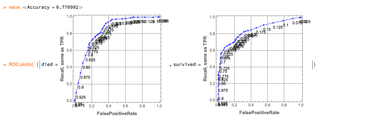

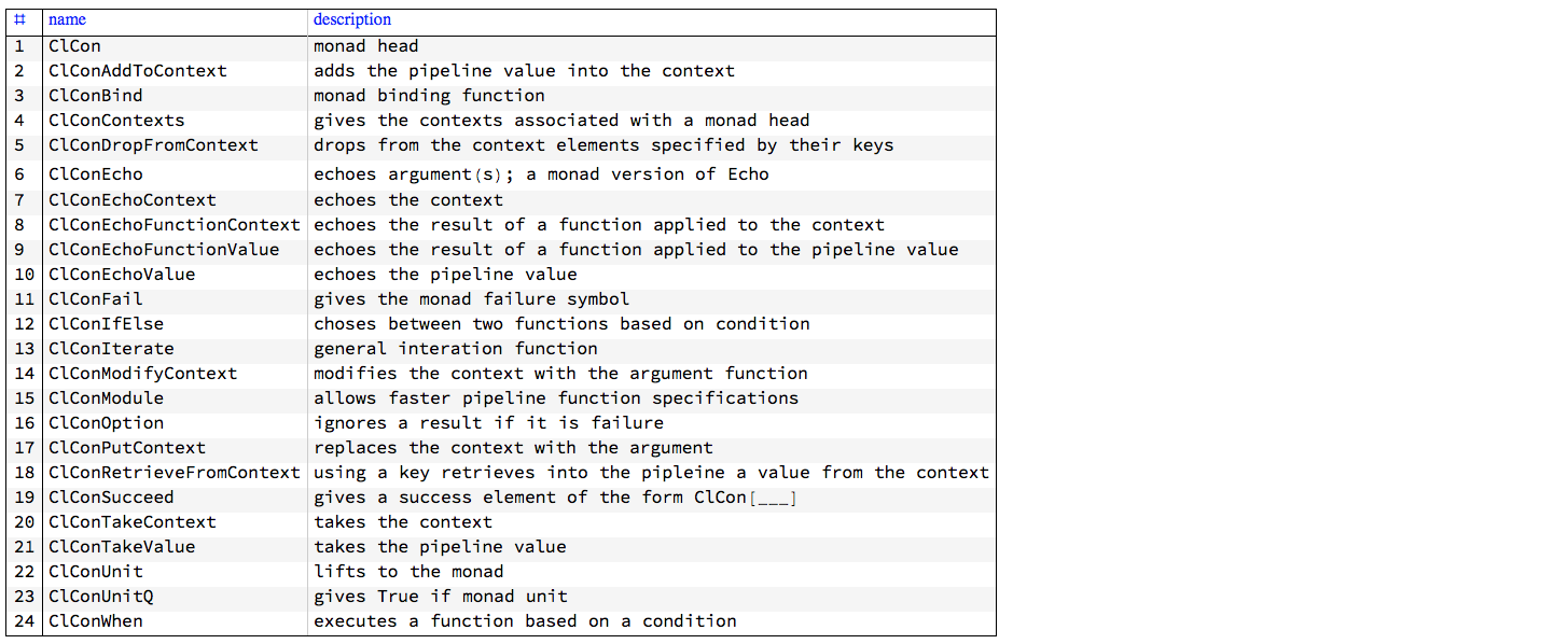


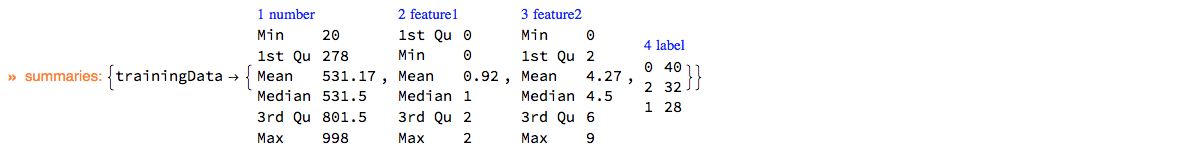


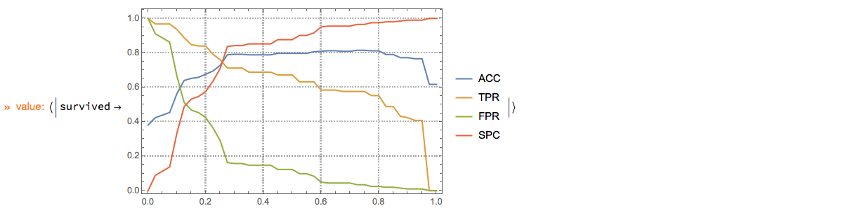


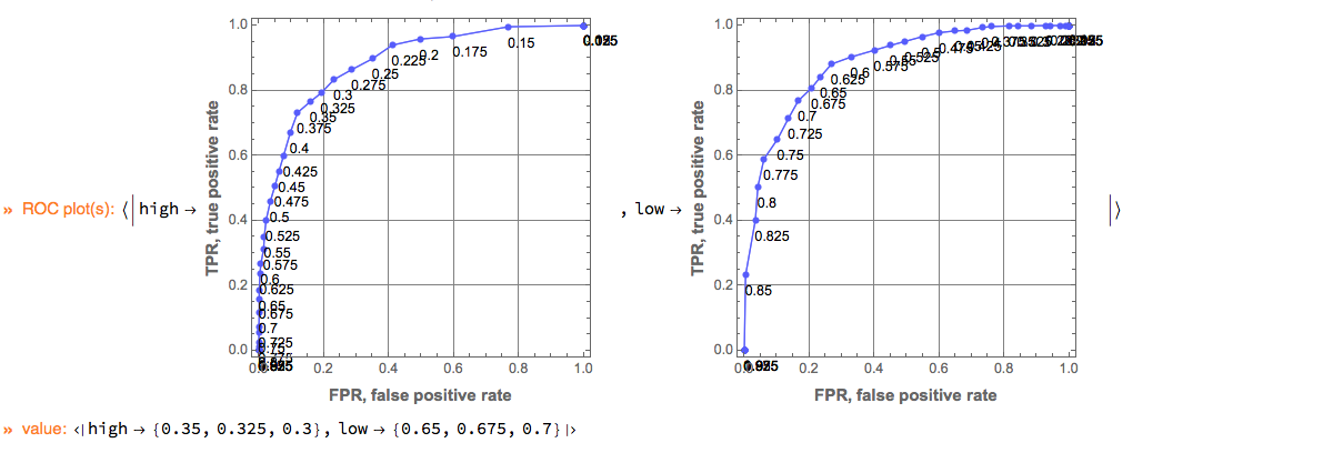


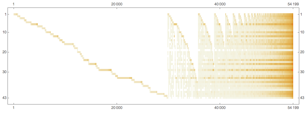


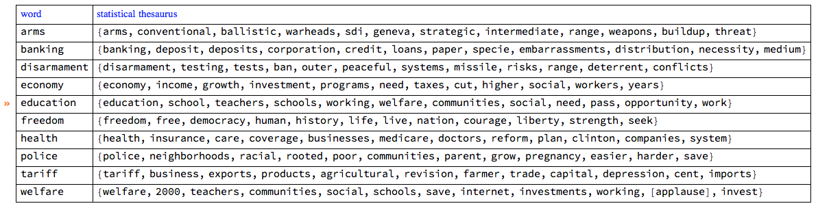

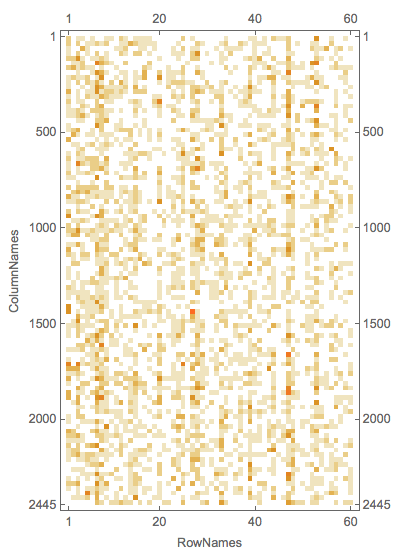
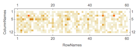

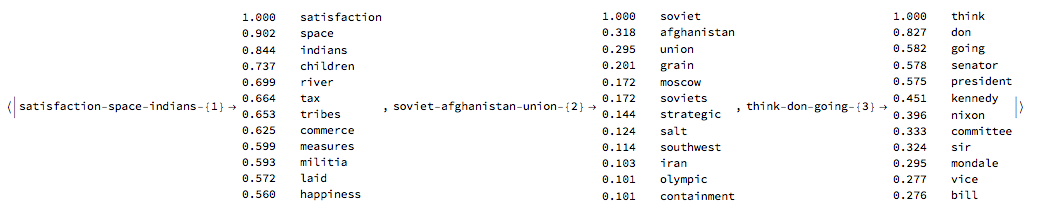

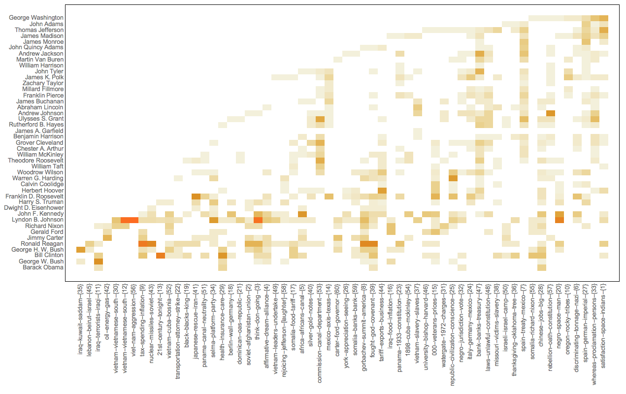
