Plenty of my concepts require point based rendering, i.e. setting millions of points on the canvas. This method sometimes works and sometimes doesn’t when using Java2D (default Processing rendering method). There is one main problem: over-saturation. This is caused by the immediate pixel blending with the canvas. Blending is done by adding color channels with weight taken from alpha and after just tens or hundreds points given pixel is fully saturated.

To fight with this issue I’ve created a small library which implements algorithm called log density mapping or rendering. The idea is based mainly on algorithms described in The Fractal Flame Algorithm paper and Physically Based Rendering code.

I will construct small log density render engine from the scratch by adding progressively all necessary features. Presented code is in Java/Processing. Each chapter has its own script.

This renderer is available also in Clojure2d library (renderer function).

To show the difference let’s compare two images: left one is created with native Java2D rendering engine, right with log density renderer.

The concept

Instead of immediate rendering of each pixel let’s define two phases.

• Accumulate number of hits and color information for given pixel
• Actual rendering of the image which calculates final color and alpha

What is important both phases are independent.

Step 0 – native rendering (CODE)

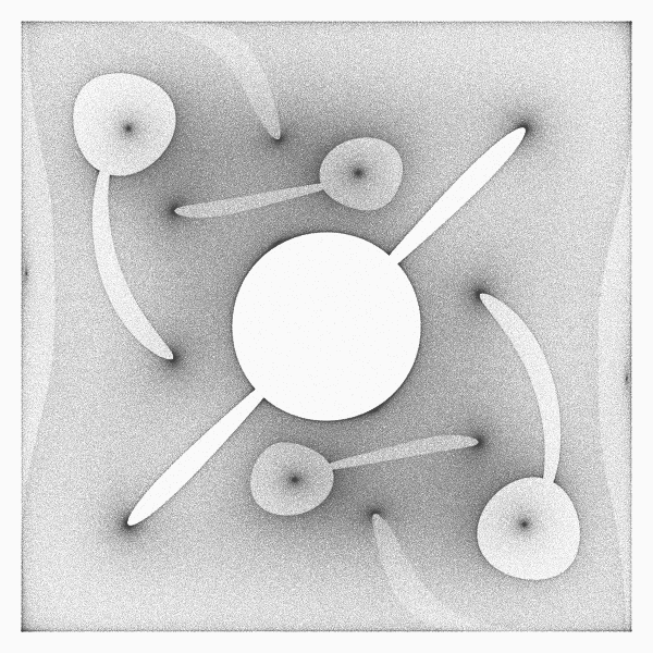
First, let’s define formula for our object: the nebula which is just 2d gaussian blob distorted by scaled perlin noise:

float noiseScale = 50.0;
PVector calcNebulaPoint() {
  float x = randomGaussian(); // take random point from gaussian distribution
  float y = randomGaussian();

  float r = noiseScale * sqrt(x*x+y*y); // calculate noise scaling factor from distance

  float nx = r * (noise(x, y) - 0.5); // shift x
  float ny = r * (noise(y-1.1, x+1.1, 0.4) - 0.5); // shift y

  return new PVector(100.0*x+nx, 100.0*y+ny);
}

To render it, just call above function milions of times with highly transparent white color.

After a while you’ll see that object saturates quickly and is losing details.

Step 1 – linear density (CODE)

Now, the simplest algorithm. When you set the pixel you need to increment number of hits for this pixel. The number of hits will determine color saturation or alpha.

To make this, we will create renderer class containing:

• array of ints – to simulate canvas and to keep number of hits for each pixel
• function which increments given pixel
• function which finally renders image

Final rendering

After adding desired number of points (say: hundreds of millions) we need to generate final image. How to convert hits into pixels? What are hits actually?

We can interpret hits as alpha channel for our pixel. At the beginning we will treat 0 as no color at all, i.e. background. Pixel with maximum hits value will be our most saturated point, i.e. white in our example. The rest values are just result of linear interpolation.

So rendering algorithm goes like that:

1. Find maximum value from all hits values
2. For each pixel, scale down hits value to 0.0 – 1.0 range
3. Set color as linear interpolation between background and most saturated color (white)

That’s all for first step. And result:

Oh yes… oh no! 😦 too dark, no details…

Gamma correction (CODE)

The main reason for that is simple: there is big gap between maximum number of hits and the rest of the image. We can try to fix it adding gamma correction in our rendering function

float alpha = pow(hits[i]/mx, 1.0/2.4); // gamma correction

Much, much better. But still not perfect, contrast seems to be low. Decreasing gamma doesn’t help, low hits pixels are now easily visible which is not good.

Step 2 – log function to the rescue (CODE)

To remove gap between low and high hits pixels let’s treat collected values as they are in log scale. This way pixels with highest hits do not differ drastically from pixels with lower number of hits.

This time gamma is equal 2.0 to darken image.

mx = log(mx+1.0); // before the loop
...
float alpha = pow(log(hits[i]+1.0)/mx,2.0);

Yes! That’s it! Contrast and brightness are ok. Low density points are barely visible. Lovely.

Indeed?

Step 3a – but… where are the colors? (CODE)

Yes, indeed, there are no colors. Till now we can only interpolate between background and foreground but it’s not enough. We need multi-color rendering. To make it we need to add more elements and collect more information.

We leave log density part as it is. Color will be collected in three arrays, each for separate color channel: red, green and blue. We will sum there color channel values.

During rendering final color is an average of collected sum of channels.

// calculate average for each channel separately
int rr = (int)(r[i]/hitsNo); // simple average
int gg = (int)(g[i]/hitsNo);
int bb = (int)(b[i]/hitsNo);

So far so good. We have colors but image is dull, dark, contrast is low. There are three tricks we can apply here.

Step 3b – better colors (CODE)

First: gamma for colors, vibrancy

Since we have gamma correction for alpha, we can introduce separate gamma correction for color channels. Additionally we can add another parameter which controls mix between calculated color (as before) and gamma corrected color. This way you can control how much gamma corrected color you want to use (0.0 – no correction, 1.0 – only gamma corrected color).

So let’s set gamma for alpha to 1.0 and gamma for color to 2.0. Below you see three results with color mix values: 0.0 (no gamma for color), 0.5 and 1.0 (full gamma for color).

Second: brightness and contrast

Operating on gamma only is not enough as you can see above. More gamma for color, darker image and necessity to decrease gamma for alpha, which can cause artifacts.

Let’s add some postprocessing for the pixel: contrast and brightness.  We’ll use algorithm from JH Labs code. There are two parameters: one controlling brightness and second controlling contrast. Value 1.0 means no change at all.

See below images for a couple of parameters combinations.

Third: saturation

To adjust color saturation we can use HSB color space. Fortunately java.awt.Color provides convenient method to convert RGB to HSB and vice versa. Adjusting is just simple multiplying by given factor. Again, value 1.0 doesn’t change anything.

All parameters:

So we have all necessary parameters to control final rendering. These are:

• gamma – gamma correction for calculated alpha channel
• cgamma – gamma correction for calculated color channels
• color_mix – ratio to control how much gamma corrected colors we want to use
• brightness
• contrast
• saturation

That’s all here.

Step 4 – what about antialiasing? (CODE)

Now the hardest part. Our method is good when we draw blobs. But sometimes aliasing artifacts may appear. How to deal with it?

There mainly two strategies: oversampling and reconstructions kernels. We will use the latter one.

Instead of setting pixel color at given position we will set “splat”. The color will be spread around given position with some weights. Then we will use sum of weights to calculate alpha and weighted average of color.

Weights are taken from kernels.

Kernels (CODE)

Reconstruction kernels are 2D functions which helps to remove higher frequencies. They blur an image a little bit, which helps to avoid aliasing artifacts.

Read more about it under following links:

• Sampling, Reconstruction, and Antialiasing
• PBRT book
• PBRT book

I prepared the tool which helps visualize all defined kernels. These are:

• Gaussian – key 0
• Windowed Sinc – key 1
• Blackman-Harris – key 2
• Triangle – key 3
• Hann – key 4

When you move mouse around you change radius (x axis) and spread (y axis) of the filter.

Pattern

Let’s render some new pattern using each filter. Pattern point is calculated as follows

float x = random(-1, 1);
float y = random(-1, 1);
float angle = atan2(y, x);
float r = 1.0+x*x+y*y;

color c = color(255*sq(sq(sin(200/r*angle))));
lr.add(400.0+x*400, 400+y*400, c);

And our image rendered with Gaussian filter

Step 5, final – multithreading (CODE)

We have all rendering elements done already. There is another aspect: speed. Although algorithm is fast enough we can improve performance and use all processor cores in for rendering.

There are three places where multithreading can be used: plotting, merging and rendering.

Till now we used one thread to add points and render result. But you can easily notice, that you can add points to separate renderers and combine all of them just by adding values from hits and color arrays. Multithreading version will work following way:

1. Create as many rendrer objects as you have processor cores
2. Run threads to plot a batch of pixels
3. Collect results and merge them into one by adding values from hits and color arrays
4. Do final rendering
5. Repeat point 2 to add more points.

What’s interesting, merging arrays and final rendering can also be run parallel.

Futures

Instead of normal threads from Processing we will use Futures. Future is a thread which can result a value when our task is finished. If it’s not finished yet, thread blocks. We don’t have to do any external synchronization. Just run, do something else and collect results (or wait and collect).

Future class and related are the part of java.util.concurrent package since Java 1.5.

I wrapped Future mechanism into Runner class in multithread.pde file. You can just copy&paste this code into your sketch and use in other cases. There are two external variables which are used: number of processor and thread pool (executor object).

int numberOfProcessors = Runtime.getRuntime().availableProcessors();
ExecutorService executor = Executors.newCachedThreadPool();

Callable

Callable is generic interface to implement when you want to create task run by Future. Type T is returning value of the task (which is just T call() function).

Drawing points

To draw points we have to create separate class for task. Each task will create it’s own rendering object, set points and return the result.

class DrawNebulaTask implements Callable {
  Renderer call() {
    Renderer lr = new Renderer(800, 800, filter); // create renderer
    drawNebula(lr, pointsNo);
    return lr;
  }
}

To run and merge result into final object we need to:

• Create Runner
• Add tasks
• Run tasks and gather results
• Merge results to the final object

As in following function

void drawAndMergeNebulas() throws InterruptedException, ExecutionException {
  Runner threads = new Runner(executor);
  for (int i=0; i<numberOfProcessors; i++) {
    threads.addTask(new DrawNebulaTask());
  }

  for (Renderer r : threads.runAndGet()) {
    buffer.merge(r);
  }
}

Merging

Merging is necessary to combine all results from separate threads into one. It’s just adding values from corresponding arrays to target. And it also can be done in parallel, each thread for each table.

private class MergeTask implements Callable {
  double[] in, buffer;

  MergeTask(double[] buffer, double[] in) {
    this.in = in;
    this.buffer = buffer;
  }

  Boolean call() {
    for (int i=0; i<in.length; i++) {
      buffer[i] += in[i];
    }
    return true;
  }
}

Rendering

Final rendering can be also refactored to multithread version. Our target PImage pixels array can be divided into separate ranges and filled by rendering function in separate threads. Check out code for details.

I measured only speed gain in this step and it’s about 3x faster than single threaded version (30ms vs 90ms)

Other concepts

There are some other elements which can be implemented here.

• Density estimation, blur low density regions to remove single pixels. Blur radius is related to density (high density – no blur, low density – wide blur radius)
• Other color spaces can be used like XYZ, LMS etc.
• Adding color channels separately to simulate chromatic abberations
• Additional weight for color to control pixel strength (semi-alpha)
• Additional gaussian spread to simulate blur.

That’s all

(To be honest I have no idea how to call this organic object).

In this article I describe how to achieve such effect. Generally speaking it’s really simple particle system with also simple attract/repel model based on love/hate attributes. This is step-by-step tutorial.

Particles

Let’s build first our basis – particles. What we need are:

• current position
• current velocity
• age – we want them to die sometimes
• color
• id – to distinguish them

And of course something to init, update and draw. First we draw them on the distorted circle. Behaviour (interactions and movement) will be the next step and will be calculated externally.

// number of particles
final static int N = 500;

// colors (some of them taken from http://www.colourlovers.com/pattern/5526827/bleak
final static color[] cols = { #FF8A00, #FFD200, #749D9D, #FCF5B3, #B39500, #272429 };

// collection of all particles
ArrayList particles = new ArrayList(N);

void setup() {
  size(800,800);
  noFill();
  smooth(8);
  strokeWeight(2.0); // exaggerate a little bit for a while
  background(0,0,20);

  // initialize particles
  for(int i=0;i<N;i++) {
   particles.add( new Particle(i) );
  }
}

void draw() {
  for(Particle p : particles) {
    p.draw();
  }
}

class Particle {
  // position
  float x,y;
  // step
  float dx, dy;
  // id
  int id;
  // life length
  float age;
  // some random color
  color c = cols[(int)random(cols.length)];

  void reset() {
    // distribute initial point on the ring, more near the outer edge, distorted
    float angle = random(TWO_PI);
    float r = 5.0*randomGaussian() + (width/2-100)*(1.0-pow(random(1.0),7.0));
    x = cos(angle)*r;
    y = sin(angle)*r;

    // set random age
    age = (int)random(100,1000);
  }

  void draw() {
   stroke(c);
   point(x+width/2,y+height/2);
  }

  // update position with externally calculated speed
  // check also age
  void update() {
    x += dx;
    y += dy;
    if(--age < 0) reset();
  }

  Particle(int i) {
    id = i;
    reset();
  }
}

Here is the initial result

Behaviour

The most important part, how we move them. Here is the only rule.

For every particle pair: if they love each other attract, reppel otherwise. That’s all.

Ok, detail is: what can be love/hate factor?

Basic love factor

The most obvious is distance. And this one is used here. Formula is

1. If distance is larger than 2.0 attract with love amount
2. Repel otherwise

Let’s see this.

// number of particles
final static int N = 500;

// colors (some of them taken from http://www.colourlovers.com/pattern/5526827/bleak
final static color[] cols = {
  #FF8A00, #FFD200, #749D9D, #FCF5B3, #B39500, #272429
};

// collection of all particles
ArrayList particles = new ArrayList(N);

void setup() {
  size(800, 800);
  noFill();
  smooth(8);
  strokeWeight(0.7);
  background(0, 0, 20);

  // initialize particles
  for (int i=0; i<N; i++) {
    particles.add( new Particle(i) );
  }
}

void draw() {
  for (Particle p : particles) {

    // love/hate vector
    float lovex = 0.0;
    float lovey = 0.0;

    for (Particle o : particles) {
      // do not compare with yourself
      if (p.id != o.id) {
        // calculate vector to get distance and direction
        PVector v = new PVector(o.x-p.x, o.y-p.y);
        float distance = v.mag();
        float angle = v.heading();

        // love!
        float love = 1.0 / distance;
        // or hate...
        if (distance<2.0) love = -love;

        // not too fast!
        love *= 0.3;

        // update love vector
        lovex += love * cos(angle);
        lovey += love * sin(angle);
      } 

      // calculated love vector will be our speed in resultant direction
      p.dx = lovex;
      p.dy = lovey;
    }
  }

  // update and draw
  for (Particle p : particles) {
   p.update();
   p.draw();
  }
}

class Particle {
  // position
  float x, y;
  // velocity
  float dx, dy;
  // id
  int id;
  // life length
  float age;
  // some random color
  color c = cols[(int)random(cols.length)];

  void reset() {
    // distribute initial point on the ring, more near the outer edge, distorted
    float angle = random(TWO_PI);
    float r = 5.0*randomGaussian() + (width/2-100)*(1.0-pow(random(1.0), 7.0));
    x = cos(angle)*r;
    y = sin(angle)*r;

    // set random age
    age = (int)random(100, 1000);
  }

  void draw() {
    stroke(c,50);
    point(x+width/2, y+height/2);
  }

  // update position with externally calculated speed
  // check also age
  void update() {
    x += dx;
    y += dy;
    if (--age < 0) reset();
  }

  Particle(int i) {
    id = i;
    reset();
  }
}

Nice, we have branching and organic look already. Our particles attract mostly, repel only when distance is low.

Attribute love factor

Now let’s introduce another attribute of our particle. It will be nonnegative floating point value . Let’s call it mood. Rule:

Our particles love each other when they have similar mood. Hate otherwise.

That means that we have to calculate similarity factor between moods to get love factor. The similarity should be between . Where means 100% love and means 100% hate. Our factor can be calculated with such formula (or something like that):

One note: don’t be strict with similarity factor, some unbalance between love and hate gives different results.

What can be mood?

• inital angle
• noise value from current position and time (mood changes while particle moves and time goes on)
• some vector field
• etc…

The code for second case as follows

// number of particles
final static int N = 500;

// colors (some of them taken from http://www.colourlovers.com/pattern/5526827/bleak
final static color[] cols = {
  #FF8A00, #FFD200, #749D9D, #FCF5B3, #B39500, #272429
};

// collection of all particles
ArrayList particles = new ArrayList(N);

void setup() {
  size(800, 800);
  noFill();
  smooth(8);
  strokeWeight(0.7);
  background(0, 0, 20);

  // initialize particles
  for (int i=0; i<N; i++) {
    particles.add( new Particle(i) );
  }
}

float time = 0.0;
void draw() {
  for (Particle p : particles) {

    // love/hate vector
    float lovex = 0.0;
    float lovey = 0.0;

    for (Particle o : particles) {
      // do not compare with yourself
      if (p.id != o.id) {
        // calculate vector to get distance and direction
        PVector v = new PVector(o.x-p.x, o.y-p.y);
        float distance = v.mag();
        float angle = v.heading();

        // love!
        float love = 1.0 / distance;
        // or hate...
        if (distance<2.0) love = -love;

        // mood factor
        love *= p.moodSimilarity(o);
        // not too fast!
        love *= 0.5;

        // update love vector
        lovex += love * cos(angle);
        lovey += love * sin(angle);
      } 

      // calculated love vector will be our speed in resultant direction
      p.dx = lovex;
      p.dy = lovey;
    }
  }

  // update and draw
  for (Particle p : particles) {
    p.update();
    p.draw();
  }

  time += 0.001;
}

class Particle {
  // position
  float x, y;
  // velocity
  float dx, dy;
  // id
  int id;
  // life length
  float age;
  // some random color
  color c = cols[(int)random(cols.length)];

  // mood factor
  float mood;

  void reset() {
    // distribute initial point on the ring, more near the outer edge, distorted
    float angle = random(TWO_PI);
    float r = 5.0*randomGaussian() + (width/2-100)*(1.0-pow(random(1.0), 7.0));
    x = cos(angle)*r;
    y = sin(angle)*r;
    // set random age
    age = (int)random(100, 2000);
    calcMood();
  }

  void draw() {
    stroke(c,50);
    point(x+width/2, y+height/2);
  }

  // update position with externally calculated speed
  // check also age
  void update() {
    if(--age < 0) {
      reset();
    } else {
      x += dx;
      y += dy;
      calcMood();
    }
  }

  Particle(int i) {
    id = i;
    reset();
  }

  // compare moods
  float moodSimilarity(Particle p) {
    return 1.0-abs(p.mood-this.mood);
  }

  // calculate current mood
  private void calcMood() {
    mood = sin(noise(x/10.0,y/10.0,time)*TWO_PI);
  }
 }

What’s next?

You can mess with several factors in this small model, eg:

• number of particles (beware, it’s )
• particle size, colors, alpha
• dinstance love/hate formulas (eg. hate distance)
• love amount (“not too fast!” comment)
• time speed
• initial position and age
• moodSimilarity and calcMood functions

Here are some examples:

 

Influences

Here are some links which guided me to this concept:

• http://www.complexification.net/gallery/machines/happyPlace/ – love/hate concept
• http://inconvergent.net/#writing – growth systems
• http://julienleonard.com/tutorials.html – growth systems
• https://ocw.mit.edu/courses/mathematics/18-177-universal-random-structures-in-2d-fall-2015/index.htm – random growth

Left to explore more deeply: random growth guided by vector field.

Enjoy!

UPDATE: Reddit elpepe5 user worked on this topic a little bit and created really nice results. Found the on GITHUB

In last article I’ve made the research about vector fields and movement based on it. This time I’m going to treat values from noise (and other functions) as acceleration.

Instead of reading an angle from noise and apply step to my drawing agents I’ll be changing angle itself and then use it in drawing step.

The code

This time drawing code looks like this. Marked line is responsible for modification of the angle.

//drawing agent
class Agent {
  PVector pos; // position of the agent
  float angle; // current angle of the agent

  void update() {
    // modify position using current angle
    pos.x += cos(angle);
    pos.y += sin(angle);

    // get point coordinates
    float xx = map(pos.x, 0, width, -1, 1);
    float yy = map(pos.y, 0, height, -1, 1);

    PVector v = new PVector(xx, yy);

    // modify an angle using noise information
    angle += map( noise(v.x, v.y), 0, 1, -1, 1);
  }
}

// all agents in the list
ArrayList<Agent> agents = new ArrayList<Agent>();

void setup() {
  size(800, 800);
  background(240);
  stroke(20, 10);
  smooth(8);
  strokeWeight(0.7);

  // initialize in random positions
  for (int i=0; i<5000; i++) {
    Agent a = new Agent();
    float posx = random(200, 600);
    float posy = random(200, 600);
    a.pos = new PVector(posx, posy);
    a.angle = random(TWO_PI);
    agents.add(a);
  }
}

float time = 0;
void draw() {
  for (Agent a : agents) {
    pushMatrix();
    // position
    translate(a.pos.x, a.pos.y);
    // rotate
    rotate(a.angle);
    // paint
    point(0, 0);
    popMatrix();
    // update
    a.update();
  }
  time += 0.001;
}

Scaling

After scaling and shifting noise I got more interesing patterns.

void update() {
  // modify position using current angle
  pos.x += cos(angle);
  pos.y += sin(angle);

  // get point coordinates
  float xx = 3 * map(pos.x, 0, width, -1, 1);
  float yy = 3 * map(pos.y, 0, height, -1, 1);

  PVector v = new PVector(xx, yy);
  v.add(new PVector(5,-3));

  // modify an angle using noise information
  angle += 3 * map( noise(v.x, v.y), 0, 1, -1, 1);
}

Applying variations

The other results can be achieved by using variations and curves described in previous articles: Folds  and Drawing vector field. Just copy them at the end of the file. Change marked line from the previous code for following code for example:

PVector v = swirl(new PVector(xx, yy),1);

Other variations produce different results and patterns.

Or something like this:

float n1 = noise(xx+5,yy-3)-0.55;

PVector vc = kampyle(n1);
PVector v = sinusoidal(vc,1);
v.mult(5);
v.add(new PVector(5,-3));

Time

As previously we can add time to get noise change during drawing. It gives nice, tissue like, objects.

angle += (3+time) * map( noise(v.x, v.y, time), 0, 1, -1, 1);

Forced movement

Another method is to add some constant value to x position in order to force movement of the points towards the right side.

Lets position all points on the left side during initialization and make number of point smaller.

// initialize in random positions
for (int i=0; i<2000; i++) {
  Agent a = new Agent();
  float posx = 100;
  float posy = random(200, 600);
  a.pos = new PVector(posx, posy);
  a.angle = random(TWO_PI);
  agents.add(a);
}

Then force movement

void update() {
  // modify position using current angle
  pos.x += cos(angle)+0.1;
  pos.y += sin(angle);

  // get point coordinates
  float xx = 3 * map(pos.x, 0, width, -1, 1);
  float yy = 3 * map(pos.y, 0, height, -1, 1);

  PVector v = new PVector(xx,yy);
  v.add(new PVector(5,-3));

  // modify an angle using noise information
  angle += (5+time) * map( noise(v.x, v.y), 0, 1, -1, 1);
}

Using some previous techniques (variations and curves) I got also such results

Or something like this.

Play and enjoy 🙂

The end

Questions? generateme.blog@gmail.com or Follow @generateme_blog

Blogs:

• GenerateMe
• Folds2d

 

folds2d.tumblr.com

The goal

During last few days I’ve made several attempts to create and visualize 2D vector fields. In the following article you can read about this concept with several examples and code in Processing.

There are many beautiful art/code based on vector field visualization around the net. Mostly based on noise function. Check them out before you start:

• Visualizer by p5art
• Furfrolic by Holger Lippmann
• My own two sketches drawing_generative and threadraw
• Few examples on OpenProcessing site: 1, 2, 3, 4

What is the vector field?

Vector field (in our case) is just a  to function exatly the same as variation described in my previous post about Folds.

Why vector? Because you can treat a pair of as vector for each point from 2d plane. This way you get field of vectors.

Vector fields can be visualised in the following way

How to get the vector field

The main goal, in this article, is to research various ways to create vector fields. There two cases.

We can operate on functions which returns pair of values like variations. In this case such function defines vector field itself. We can use also some vector operations (like substraction, sum, etc…) to get new functions.

The second option is to get single float number like from noise(), dist() between points or dot product of vectors, etc. And convert this number into vector.

Drawing method

The method is quite simple.

1. Create points from  floating point range
2. Draw them
3. For each of the point calculate relating vector from the vector field
4. Scale it and add to the point coordinates
5. Repeat 2-4

Step 4 is key here. We move our points along vectors. Trace lines build the resulting image.

The general flow for constructing vector field follows this scheme:

Note: I assume that on every step I can multiply function variables or returned values by any number.

Here is code stub for my experiments

// dynamic list with our points, PVector holds position
ArrayList<PVector> points = new ArrayList<PVector>();

// colors used for points
color[] pal = {
  color(0, 91, 197),
  color(0, 180, 252),
  color(23, 249, 255),
  color(223, 147, 0),
  color(248, 190, 0)
};

// global configuration
float vector_scale = 0.01; // vector scaling factor, we want small steps
float time = 0; // time passes by

void setup() {
  size(800, 800);
  strokeWeight(0.66);
  background(0, 5, 25);
  noFill();
  smooth(8);

  // noiseSeed(1111); // sometimes we select one noise field

  // create points from [-3,3] range
  for (float x=-3; x<=3; x+=0.07) {
    for (float y=-3; y<=3; y+=0.07) {
      // create point slightly distorted
      PVector v = new PVector(x+randomGaussian()*0.003, y+randomGaussian()*0.003);
      points.add(v);
    }
  }
}

void draw() {
  int point_idx = 0; // point index
  for (PVector p : points) {
    // map floating point coordinates to screen coordinates
    float xx = map(p.x, -6.5, 6.5, 0, width);
    float yy = map(p.y, -6.5, 6.5, 0, height);

    // select color from palette (index based on noise)
    int cn = (int)(100*pal.length*noise(point_idx))%pal.length;
    stroke(pal[cn], 15);
    point(xx, yy); //draw

    // placeholder for vector field calculations

    // v is vector from the field
    PVector v = new PVector(0, 0);

    p.x += vector_scale * v.x;
    p.y += vector_scale * v.y;

    // go to the next point
    point_idx++;
  }
  time += 0.001;
}

When I change my field vector to be constant one (different than 0), my points start move.

PVector v = new PVector(0.1, 0.1);

Perlin noise

Let’s begin with perlin noise in few configurations. I’m going to change only marked lines from the code stub.

Variant 1

noise(x,y) function in processing returns value from 0 to 1 (actually implementation used in Processing has some problems and real value is often in range from 0.2 to 0.8). I will treat resulted value as an angle in polar coordinates and use sin()/cos() functions to convert it to cartesian ones. To properly do this I have to scale it up to range or or even more. I show few variants here.

// placeholder for vector field calculations
float n = TWO_PI * noise(p.x,p.y);
PVector v = new PVector(cos(n),sin(n));

Variant 2

Let’s check what happens when I multiply noise by 10, 100, 300 or even 1000. Noise is now scaled to range (it is more usable range in further examples).

float n = 10 * map(noise(p.x/5,p.y/5),0,1,-1,1); // 100, 300 or 1000
PVector v = new PVector(cos(n),sin(n));

Variant 3

Two of above variants were using classic method. Now I get rid of polar->cartesian conversion and I’m going to treat returned value from noise() as cartesian coordinates. Angle of the vector is the same for whole field and only length of vector is changed. This leads to some interesting patterns. Experiment with scaling input coordinates and

 

float n = 5*map(noise(p.x,p.y),0,1,-1,1);
PVector v = new PVector(n,n);

Parametric curves

Let’s use parametric curves to convert noise() result into vector. The big list of them is defined in Wolfram Alpha or named here. Parametric curve (or plane curve) is a function . Click section name to see plot of the curve.

 

Astroid

// placeholder for vector field calculations
float n = 5*map(noise(p.x,p.y),0,1,-1,1); // and 2

float sinn = sin(n);
float cosn = cos(n);

float xt = sq(sinn)*sinn;
float yt = sq(cosn)*cosn;

PVector v = new PVector(xt,yt);

Results for noise scale 2 and 5

Cissoid of Diocles

// placeholder for vector field calculations
float n = 3*map(noise(p.x,p.y),0,1,-1,1);

float sinn2 = 2*sq(sin(n));

float xt = sinn2;
float yt = sinn2*tan(n);

PVector v = new PVector(xt,yt);

Kampyle of Eudoxus

// placeholder for vector field calculations
float n = 6*map(noise(p.x,p.y),0,1,-1,1);

float sec = 1/sin(n);

float xt = sec;
float yt = tan(n)*sec; 

PVector v = new PVector(xt,yt);

Rectangular Hyperbola

// placeholder for vector field calculations
float n = 10*map(noise(p.x*2,p.y*2),0,1,-1,1);

float xt = 1/sin(n);
float yt = tan(n); 

PVector v = new PVector(xt,yt);

Superformula

// placeholder for vector field calculations
float n = 5*map(noise(p.x,p.y),0,1,-1,1);

float a = 1;
float b = 1;
float m = 6;
float n1 = 1;
float n2 = 7;
float n3 = 8;

float f1 = pow(abs(cos(m*n/4)/a),n2);
float f2 = pow(abs(sin(m*n/4)/b),n3);
float fr = pow(f1+f2,-1/n1);

float xt = cos(n)*fr;
float yt = sin(n)*fr;

PVector v = new PVector(xt,yt);

Noise and curves combined

Now I’m going to play with some combinations of above curves and make multiple passes through noise().

Let’s put all curves into functions (paste following code to the end of the script):

PVector circle(float n) { // polar to cartesian coordinates
  return new PVector(cos(n), sin(n));
}

PVector astroid(float n) {
  float sinn = sin(n);
  float cosn = cos(n);

  float xt = sq(sinn)*sinn;
  float yt = sq(cosn)*cosn;

  return new PVector(xt, yt);
}

PVector cissoid(float n) {
  float sinn2 = 2*sq(sin(n));

  float xt = sinn2;
  float yt = sinn2*tan(n);

  return new PVector(xt, yt);
}

PVector kampyle(float n) {
  float sec = 1/sin(n);

  float xt = sec;
  float yt = tan(n)*sec;

  return new PVector(xt, yt);
}

PVector rect_hyperbola(float n) {
  float sec = 1/sin(n);

  float xt = 1/sin(n);
  float yt = tan(n);

  return new PVector(xt, yt);
}

final static float superformula_a = 1;
final static float superformula_b = 1;
final static float superformula_m = 6;
final static float superformula_n1 = 1;
final static float superformula_n2 = 7;
final static float superformula_n3 = 8;
PVector superformula(float n) {
  float f1 = pow(abs(cos(superformula_m*n/4)/superformula_a), superformula_n2);
  float f2 = pow(abs(sin(superformula_m*n/4)/superformula_b), superformula_n3);
  float fr = pow(f1+f2, -1/superformula_n1);

  float xt = cos(n)*fr;
  float yt = sin(n)*fr;

  return new PVector(xt, yt);
}

Variant 1 – p5art

Code based on p5art web app noisePainting

// placeholder for vector field calculations
float n1 = 10*noise(1+p.x/20, 1+p.y/20); // shift input to avoid symetry
float n2 = 5*noise(n1, n1);
float n3 = 325*map(noise(n2, n2), 0, 1, -1, 1); // 25,325

PVector v = circle(n3);

Variant 2

// placeholder for vector field calculations
float n1 = 15*map(noise(1+p.x/20, 1+p.y/20),0,1,-1,1);

PVector v1 = cissoid(n1);
PVector v2 = astroid(n1);

float n2a = 5*noise(v1.x,v2.y);
float n2b = 5*noise(v2.x,v1.y);

float n3 = 10*map(noise(n2a, n2b/3), 0, 1, -1, 1);

PVector v = circle(n3);

Variant 3

// placeholder for vector field calculations
float n1 = 15*map(noise(1+p.x/10, 1+p.y/10),0,1,-1,1);

PVector v1 = rect_hyperbola(n1);
PVector v2 = astroid(n1);

float n2a = 2*map(noise(v1.x,v1.y),0,1,-1,1);
float n2b = 2*map(noise(v2.x,v2.y),0,1,-1,1);

PVector v = new PVector(n2a,n2b);

Variant 4

// placeholder for vector field calculations
PVector v1 = kampyle(p.x);
PVector v2 = superformula(p.y);

float n2a = 3*map(noise(v1.x,v1.y),0,1,-1,1);
float n2b = 3*map(noise(v2.x,v2.y),0,1,-1,1);

PVector v = new PVector(cos(n2a),sin(n2b));

Variant 5

// placeholder for vector field calculations
float n1a = 3*map(noise(p.x,p.y),0,1,-1,1);
float n1b = 3*map(noise(p.y,p.x),0,1,-1,1);

PVector v1 = rect_hyperbola(n1a);
PVector v2 = astroid(n1b);

float n2a = 3*map(noise(v1.x,v1.y),0,1,-1,1);
float n2b = 3*map(noise(v2.x,v2.y),0,1,-1,1);

PVector v = new PVector(cos(n2a),sin(n2b));

Variant 6 – comparison

Here I want to compare different curves using the same method. I change marked lines into pair of curves defined above. I’ve put noiseSeed(1111); in setup() to have the same noise structure. Check image description to see what curves were used.

// placeholder for vector field calculations
float n1a = 15*map(noise(p.x/10,p.y/10),0,1,-1,1);
float n1b = 15*map(noise(p.y/10,p.x/10),0,1,-1,1);

PVector v1 = superformula(n1a);
PVector v2 = circle(n1b);

PVector diff = PVector.sub(v2,v1);
diff.mult(0.3);

PVector v = new PVector(diff.x,diff.y);

Time

Now let’s introduce time. An external variable which is incremented every frame with some small value. It can be used to slightly change noise field during rendrering or can be used as a scale factor.

Let’s compare the same vector field without time and time used as third noise parameter.

 // placeholder for vector field calculations
 float n1a = 3*map(noise(p.x/2,p.y/2),0,1,-1,1);
 float n1b = 3*map(noise(p.y/2,p.x/2),0,1,-1,1);
 float nn = 6*map(noise(n1a,n1b),0,1,-1,1);

 PVector v = circle(nn);

And now I add time as a third parameter to noise function. This way our vector field changes when time passes.

 // placeholder for vector field calculations
float n1a = 3*map(noise(p.x/2,p.y/2,time),0,1,-1,1);
float n1b = 3*map(noise(p.y/2,p.x/2,time),0,1,-1,1);
float nn = 6*map(noise(n1a,n1b,time),0,1,-1,1);

PVector v = circle(nn);

Now time is used as a scaling factor.

// placeholder for vector field calculations
float n1a = 3*map(noise(p.x/2,p.y/2),0,1,-1,1);
float n1b = 3*map(noise(p.y/2,p.x/2),0,1,-1,1);

float nn = time*10*6*map(noise(n1a,n1b),0,1,-1,1);

PVector v = circle(nn);

Variations

Now let’s introduce variations (see previous post about Folds) as a vector field definition.

Copy below code to the end of your sketch. It includes function definiotions used in this and next chapters.

PVector sinusoidal(PVector v, float amount) {
  return new PVector(amount * sin(v.x), amount * sin(v.y));
}

PVector waves2(PVector p, float weight) {
  float x = weight * (p.x + 0.9 * sin(p.y * 4));
  float y = weight * (p.y + 0.5 * sin(p.x * 5.555));
  return new PVector(x, y);
}

PVector polar(PVector p, float weight) {
  float r = p.mag();
  float theta = atan2(p.x, p.y);
  float x = theta / PI;
  float y = r - 2.0;
  return new PVector(weight * x, weight * y);
}

PVector swirl(PVector p, float weight) {
  float r2 = sq(p.x)+sq(p.y);
  float sinr = sin(r2);
  float cosr = cos(r2);
  float newX = 0.8 * (sinr * p.x - cosr * p.y);
  float newY = 0.8 * (cosr * p.y + sinr * p.y);
  return new PVector(weight * newX, weight * newY);
}

PVector hyperbolic(PVector v, float amount) {
  float r = v.mag() + 1.0e-10;
  float theta = atan2(v.x, v.y);
  float x = amount * sin(theta) / r;
  float y = amount * cos(theta) * r;
  return new PVector(x, y);
}

PVector power(PVector p, float weight) {
  float theta = atan2(p.y, p.x);
  float sinr = sin(theta);
  float cosr = cos(theta);
  float pow = weight * pow(p.mag(), sinr);
  return new PVector(pow * cosr, pow * sinr);
}

PVector cosine(PVector p, float weight) {
  float pix = p.x * PI;
  float x = weight * 0.8 * cos(pix) * cosh(p.y);
  float y = -weight * 0.8 * sin(pix) * sinh(p.y);
  return new PVector(x, y);
}

PVector cross(PVector p, float weight) {
  float r = sqrt(1.0 / (sq(sq(p.x)-sq(p.y)))+1.0e-10);
  return new PVector(weight * 0.8 * p.x * r, weight * 0.8 * p.y * r);
}

PVector vexp(PVector p, float weight) {
  float r = weight * exp(p.x);
  return new PVector(r * cos(p.y), r * sin(p.y));
}

// parametrization P={pdj_a,pdj_b,pdj_c,pdj_d}
float pdj_a = 0.1;
float pdj_b = 1.9;
float pdj_c = -0.8;
float pdj_d = -1.2;
PVector pdj(PVector v, float amount) {
  return new PVector( amount * (sin(pdj_a * v.y) - cos(pdj_b * v.x)),
  amount * (sin(pdj_c * v.x) - cos(pdj_d * v.y)));
}

final float cosh(float x) { return 0.5 * (exp(x) + exp(-x));}
final float sinh(float x) { return 0.5 * (exp(x) - exp(-x));}

Let’s see how individual variations look as vector fields. Sometimes I had to adjust scaling factor to keep points on the screen.

// placeholder for vector field calculations
PVector v = sinusoidal(p,1);
v.mult(1); // different values for different functions

All together

Let’s sumarize what functions we have now defined.

• 
  • multiplying/dividing by number
  • single variable noise()
  • other single variable functions (sin/cos, exp, log, sq, sqrt, etc.)
• 
  • parametric curves
• 
  • noise() with two parameters
  • distance between vectors
  • dot product of vectors
  • length of the vector
  • angle between vectors
• 
  • variations and their combinations
  • sum or difference of vectors
  • atan2() of the vector

All above operations can be used to generate vector field (or simply transform 2d point to another 2d point).

I will play with above transformations in following examples. It’s a record of experiments.

Variant 1

// placeholder for vector field calculations
float n1 = 5*map(noise(p.x/5,p.y/5),0,1,-1,1);

PVector v1 = rect_hyperbola(n1);
PVector v2 = swirl(v1,1);

PVector v = new PVector(cos(v2.x),sin(v2.y));

Variant 2

// placeholder for vector field calculations
float n1 = 5*map(noise(p.x/5,p.y/5),0,1,-1,1);
float n2 = 5*map(noise(p.y/5,p.x/5),0,1,-1,1);

PVector v1 = vexp(new PVector(n1,n2),1);
PVector v2 = swirl(new PVector(n2,n1),1);

PVector v3 = PVector.sub(v2,v1);

PVector v4 = waves2(v1,1);
v4.mult(0.8);

PVector v = new PVector(v4.x,v4.y);

Variant 3

// placeholder for vector field calculations
PVector v1 = vexp(p,1);

float n1 = map(noise(v1.x,v1.y,time),0,1,-1,1);
float n2 = map(noise(v1.y,v1.x,-time),0,1,-1,1);

PVector v2 = vexp(new PVector(n1,n2),1);

PVector v = new PVector(v2.x,v2.y);

Variant 4

// placeholder for vector field calculations
PVector v1 = polar(cross(p,1),1);

float n1 = 15*map(noise(v1.x,v1.y,time),0,1,-1,1);
PVector v2 = cissoid(n1);
v2.normalize();

PVector v = new PVector(v2.x,v2.y);

Variant 5

// placeholder for vector field calculations
PVector v1 = power(p,1);

float n1 = 5*map(noise(v1.x,v1.y,time),0,1,-1,1);
float n2 = 5*map(noise(p.x/3,p.y/3,-time),0,1,-1,1);

PVector v2 = cosine(new PVector(n1,n2),1);

float a1 = PVector.angleBetween(v1,v2);

PVector v3 = superformula(a1);
v3.mult(3);

PVector v = new PVector(cos(v3.x),sin(v3.y));

Variant 6

// placeholder for vector field calculations
PVector v1 = waves2(p,1);
PVector v2 = PVector.sub(v1,p);

float n1 = 8*noise(time)*atan2(v1.y,v1.x);
float n2 = 8*noise(time+0.5)*atan2(v2.y,v2.x);

PVector v = new PVector(cos(v2.x*n1),sin(v1.y+n2));

Variant 7

// placeholder for vector field calculations
PVector v1 = swirl(p,1);
v1.mult(0.5);
PVector v2 = PVector.sub(v1,p);

float nv1 = noise(v1.x,v1.y,time);
float nv2 = noise(v2.x,v2.y,-time);

float n1 = (atan2(v1.y,v1.x)+nv2);
float n2 = (atan2(v2.y,v2.x)+nv1);

PVector v3 = superformula(n1);
PVector v4 = rect_hyperbola(n2);

PVector tv3 = waves2(v3,1);
PVector tv4 = sinusoidal(v4,1);

PVector v5 = PVector.sub(tv4,tv3);

PVector v6 = pdj(v5,1);

float an = PVector.angleBetween(v6,new PVector(n1,n2));

PVector v = new PVector(cos(v2.x+sin(an)),sin(v6.y-cos(an)));
v.mult(1+time*40);

Image

The last part is about using channel information from an image as a vector field. I wrote two sketches some time ago which are based on vector field concept.

Drawing generative

Threadraw

How to use image data

First load your image at the beginning of the sketch

img = loadImage("natalie.jpg"); // PImage img; must be declared globally

Then use image data following way

// placeholder for vector field calculations
PVector v1 = sinusoidal(p,1);

int img_x = (int)map(p.x,-3,3,0,img.width);
int img_y = (int)map(p.y,-3,3,0,img.height);

float b = brightness( img.get(img_x,img_y) )/255.0;
PVector br = circle(b);

float a = 5*PVector.angleBetween(br,v1);

PVector v = astroid(a);

Appendix

This concept is taken from zach lieberman and Keith Peters who explored painting by non-intersecting segments. This idea can be used on vector fields too. Here are two examples.

See the code HERE.

The end

Questions? generateme.blog@gmail.com or Follow @generateme_blog