<?xml version="1.0" encoding="utf-8"?><feed xmlns="http://www.w3.org/2005/Atom" ><generator uri="https://jekyllrb.com/" version="3.10.0">Jekyll</generator><link href="https://gaborvecsei.com/feed.xml" rel="self" type="application/atom+xml" /><link href="https://gaborvecsei.com/" rel="alternate" type="text/html" /><updated>2026-01-19T08:39:02+00:00</updated><id>https://gaborvecsei.com/feed.xml</id><title type="html">Gábor Vecsei</title><subtitle>Personal webpage</subtitle><entry><title type="html">Fog and the balcony - wide crops from photos</title><link href="https://gaborvecsei.com/fog-and-the-balcony-gallery/" rel="alternate" type="text/html" title="Fog and the balcony - wide crops from photos" /><published>2022-12-09T00:00:00+00:00</published><updated>2022-12-09T00:00:00+00:00</updated><id>https://gaborvecsei.com/fog-and-the-balcony-gallery</id><content type="html" xml:base="https://gaborvecsei.com/fog-and-the-balcony-gallery/"><![CDATA[]]></content><author><name>gaborvecsei</name></author><category term="blog" /><category term="Art" /><category term="Photography" /><category term="Pixel7Pro" /><summary type="html"><![CDATA[]]></summary></entry><entry><title type="html">Neural Network Steganography</title><link href="https://gaborvecsei.com/Neural-Network-Steganography/" rel="alternate" type="text/html" title="Neural Network Steganography" /><published>2022-05-20T00:00:00+00:00</published><updated>2022-05-20T00:00:00+00:00</updated><id>https://gaborvecsei.com/Neural-Network-Steganography</id><content type="html" xml:base="https://gaborvecsei.com/Neural-Network-Steganography/"><![CDATA[<h1 id="introduction">Introduction</h1>

<p><em>We all have secrets, and now you can share these with your favorite neural network</em> 🤫</p>

<p><a href="https://github.com/gaborvecsei/Neural-Network-Steganography">gaborvecsei/Neural-Network-Steganography - <strong>Code and notebooks for the experiments</strong></a>.
I encourage everybody to follow the post with the code for easier and more practical understanding.</p>

<p>Steganography is the practice of concealing a message within another message or a physical object <a href="#references"><em>[1]</em></a>.
Hiding a message in a picture, or a picture within another picture are good examples on how you can break down the
two entities (what we can call <em>base data</em> and <em>secret data</em>) and slightly alter the base to hide your secret.
The idea, is that you can make really small
modifications to the base which is usually impossible to spot with your eyes and those modifications contain what you
wanted to hide.</p>

<blockquote>
  <p>Imagine increasing every $R$ value from the $(R, G, B)$ representation of the image with $1$ if $R &lt; 255$.
The result is a brand new image where you’ve hidden your “secret”, and still you will hardly be able to tell them apart.</p>
</blockquote>

<p>The idea is the same with neural networks as a NN can contain millions of parameters which we can smartly modify to
embed some secrets.
This is what we can read about in the publication <em>“EvilModel: Hiding Malware Inside of Neural Network Models”</em> <a href="#references"><em>[2]</em></a>
which I wanted to test with my own implementation.</p>

<h1 id="floating-points-and-how-to-modify-them">Floating-Points and how to modify them</h1>

<p>In computer science, we are only approximating real numbers as you’d need infinite bits to represent a real number
with infinite precision. This is why we are using the floating-point numbers with which we can represent these numbers
with a fixed number of bits to a certain precision and range.
In this post I will be using the single precision, 32 bit representation (<code class="language-plaintext highlighter-rouge">float32</code>), but you could easily extend the theory
for representations with more/fewer bits.</p>

<h2 id="structure-of-a-fp32">Structure of a FP32</h2>

<p>I won’t cover the whole story around floating points, there are several well written articles, you can read it up here: <a href="#references"><em>[3]</em></a>,
but as a quick refresher, this is what you need to know for these experiments.
We can split the binary representation into 3 parts and then use these to calculate the value of the number:</p>
<ul>
  <li><em>sing</em> ($s$) - the 1st bit</li>
  <li><em>exponent</em> ($E$) - 8 bits after the sign bit</li>
  <li><em>fraction</em> ($F$) - 23 bits after the last bit of the exponent</li>
</ul>

<p><img src="https://upload.wikimedia.org/wikipedia/commons/thumb/d/d2/Float_example.svg/885px-Float_example.svg.png" width="400" alt="" /></p>

<p>(<em>LSB</em> visualization, source: <a href="#references"><em>[3]</em></a>)</p>

<p>Modifying these binary representations allows us to store some data while giving up some precision what we can control by
the decision how many and which bits to change in the original bit sequence.
The formula to calculate the real number is from which we can see that by modifying $F$ we can do the least harm <a href="#references"><em>[6]</em></a>:</p>

<p>$x = (-1)^s \times (1.F) \times 2^{E-127}$</p>

<h2 id="floating-point-experiment">Floating-Point experiment</h2>

<p>As an experiment, let’s say, we would like to modify the number $x=-69.420$. I wrote a little utility class <a href="#references"><em>[4]</em></a> with which we
can easily experiment with the representation.
Let’s take $x$, convert to the mentioned
binary representation: $11000010100010101101011100001010$ and then calculate it’s value again with the formula: $-69.41999816894531$.
It’s not the same as the original one…🤔 and yeah that’s the whole point, the difference is $1.8310546892053026e-06$.
And kids, this is why we are not doing <del>drugs</del> equality checks with floats.</p>

<p>As another experiment we can take $16bits$ from the fraction of $x$ and play around with it, “simulate” how the value changes as we change these bits.
Randomly doing this $1000$ times yields the following plot:</p>

<p><img src="https://gaborvecsei.github.io/assets/images/blog/nn_steganography/fp32_modification_randomly.png" width="400" alt="" /></p>

<p>But of course we can just set all bits to $0$s and $1$s and then we have the “range of change”.
The wider this range is the more afraid we should be when modifying the NN, as predictions can and will be altered.</p>

<p>You can also experiment more with <code class="language-plaintext highlighter-rouge">float32</code>s just <a href="https://github.com/gaborvecsei/Neural-Network-Steganography/blob/master/float_investigation.ipynb">run this notebook</a>.</p>

<h1 id="hiding-the-secrets-in-neural-networks">Hiding the secrets in Neural Networks</h1>

<p>The process is the following:</p>

<ol>
  <li>🔎 Evaluate your NN without any modification on a test dataset
    <ul>
      <li>Store each individual prediction not just the overall metrics (e.g. f1 score) - for more through evaluation</li>
    </ul>
  </li>
  <li>0️⃣1️⃣ Convert your data/secret to binary representation</li>
  <li>🤓 Calculate how many bits are needed to hide this data, then check if you have the available “storage” in your NN
    <ul>
      <li>$storage=\text{nb_bits} * \text{nb_parameters}$</li>
      <li>Remember that there is a quality-quantity trade-off so try to use low number of bits</li>
    </ul>
  </li>
  <li>🤖Go over the parameters in the network, convert to binary format, then switch the defined bits to bits from the secret</li>
  <li>🔎 Evaluate the NN again, and inspect the differences</li>
</ol>

<h2 id="quality---quantity-trade-off">Quality - Quantity trade-off</h2>

<p>There is a trade-off what we need to consider when modifying bits of parameters in a neural network:
The more precision you give up at each value the more data you can store.
But think about what this precision means in a NN.
You are using these parameters to perform the forward pass and receive a prediction, and you’d like to keep this prediction as close as you can to the original one.
Worst case scenario, the outputs of the network will be so different, that you won’t notice the 24 days of training what you did.</p>

<p>As a general rule, just try to compress your data and use less bits from the fraction.
Empirically it’s better to modify less bits everywhere int he network compared to modify more bits for certain selected layers.
I will include such measurements in upcoming posts.</p>

<h2 id="experiment">Experiment</h2>

<p>After all this theory let’s see an actual experiment 🥳.
I wrote the tools to use it not just to sit on it 🦾.</p>

<h3 id="parameters">Parameters</h3>

<p>I used the well known <code class="language-plaintext highlighter-rouge">ResNet50</code> network trained on <code class="language-plaintext highlighter-rouge">ImageNet</code> which is easily accessible at every deep learning framework.
But how much data can we store here? Actually… a lot, but it should not be surprising with the number of parameters.
After I decided to run the experiment, where I change $16bits$ from the <em>fraction</em> of every parameter (in every <code class="language-plaintext highlighter-rouge">Conv2D</code> layer) I could calculate the amount of data I can store.
Here you can see the layer-wise breakdown:</p>

<p><img src="https://gaborvecsei.github.io/assets/images/blog/nn_steganography/resnet50_conv2d_storage_capacity.png" width="640" alt="" /></p>

<p>
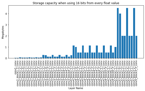
Adding up all the bits for the params in the 53 layers, it turns out we can easily store $44MB$s of data.
And keep in mind that today this is an averaged size CV model.
It would be really easy to hide a few Trojan viruses here <a href="#references"><em>[5]</em></a>.</p>

<p>We can also take a look on basic statistics for the parameters, to get a hint how much precision we need to retain, and
these would help for any fancier placement of the secret bits (e.g. Calculate the number of bits to use for clusters on values), but I will be using a simple iterative method.</p>

<div class="language-plaintext highlighter-rouge"><div class="highlight"><pre class="highlight"><code>Min: -0.7719802856445312
Abs. Min: 8.192913014681835e-10
Max: 0.9003667831420898
Mean: -0.0007807782967574894
---
Nb total values: 23454912
Nb values &lt; 10e-4: 1486452 - 6.3375%
Nb values &lt; 10e-3: 13138630 - 56.0165%
Nb negatives: 12746193 - 54.3434%
Nb positives: 10708719 - 45.6566%
---
(Maximum) Storage capacity is 44.0 MB for the 53 layers with the 16 bits modification
</code></pre></div></div>

<h3 id="placement-of-the-bits">Placement of the bits</h3>

<p>For quick experimentation I chose to generate a random $44MB$ data as a secret and a simple iterative approach for hiding it,
where I use a stepping window on the secret bits and starting from the 1st layers 1st parameter I make the modifications.
In the first iteration I take the bits from 0th to 15th from the secret, convert the first parameter in the first <code class="language-plaintext highlighter-rouge">conv2d</code> layer to the binary representation,
take the last 16 bits of the fraction and switch the two. The second iteration I step the window and take it from 16th to 31th and switch with the last 16 bits of the second parameter.
And this goes on until we don’t have any more bits to hide.</p>

<h3 id="reconstruction">Reconstruction</h3>

<p>So I think the backward process is obvious and I won’t waste virtual paper on it (it’s a homework for everyone reading this 😉),
but there are 3 things you need to remember for the reconstruction:</p>
<ul>
  <li>The order in which you modified the layers and the parameters (now it’s ordered by the index of the layer in the NN)</li>
  <li>The number of bits used for each parameter (fortunately it’s global for this algo)</li>
  <li>The index of the last modified parameter, so we can stop the process
    <ul>
      <li>(If your data is $8 bits$ while your NN has $20,000,000$ parameters, you can hide a single bit in the first $8$ parameters)</li>
    </ul>
  </li>
</ul>

<h3 id="evaluation---how-much-the-predictions-changed">Evaluation - How much the predictions changed?</h3>

<p>As the test dataset I used images randomly found on my laptop, as we don’t necessarily interested in the predictions,
only in the difference of the predictions compared to the original state. You only need to pay attention that the
dataset should be diverse enough, so it covers all cases the network can meet with.</p>

<p>With my $14,241$ images the results are the following:</p>

<p>Analyzing the <em>softmax</em> output values with the 1000 classes:</p>

<div class="language-plaintext highlighter-rouge"><div class="highlight"><pre class="highlight"><code>Min abs difference: 0.0
Max abs difference: 0.11202079057693481
Number of changed prediction values: 14240972 / 14241000 | 99.9998%
</code></pre></div></div>

<p>Looking only at the changes where the prediction label (<code class="language-plaintext highlighter-rouge">np.argmax(output)</code>) is different:</p>

<div class="language-plaintext highlighter-rouge"><div class="highlight"><pre class="highlight"><code>Changed number of predictions: 146 / 14241 | 1.0252089038691103%
</code></pre></div></div>

<p>So we can see that almost all outputs changed slightly, and for some cases (approx. $1\%$) this resulted in a new output label.
This is not surprising based on the maximum change values, just imagine a 3 class case where these are the original values:
$[0.3, 0.34, 0.36]$ (label would be <em>2</em>) and after the modification it’s: $[0.3, 0.351, 0.349]$ (where label is <em>1</em>).</p>

<h1 id="conclusion">Conclusion</h1>

<p>While using a relatively simple approach it is clear that we can use NNs to hide secrets. A lot of secrets…
With keeping in mind the introduced trade-offs, and testing of the approaches, we can modify the network while loosing little accuracy.</p>

<p>I think you are already thinking about smarter and more sophisticated approaches, and in a follow up I would like to test those,
and evaluate a wider range of models.</p>

<h1 id="references">References</h1>

<p><em>[1]</em> - <a href="https://en.wikipedia.org/wiki/Steganography">Steganography - Wikipedia</a></p>

<p><em>[2]</em> - <a href="https://arxiv.org/abs/2107.08590">EvilModel: Hiding Malware Inside of Neural Network Models</a></p>

<p><em>[3]</em> - <a href="https://en.wikipedia.org/wiki/Single-precision_floating-point_format">Single-precision floating-point format - Wikipedia</a></p>

<p><em>[4]</em> - <a href="https://github.com/gaborvecsei/Neural-Network-Steganography/blob/master/float_investigation.ipynb">Floating point investigation notebook</a></p>

<p><em>[5]</em> - <a href="https://nakedsecurity.sophos.com/2010/07/27/large-piece-malware/#">How large is a piece of Malware? - SophosLabs</a></p>

<p><em>[6]</em> - <a href="https://www.sciencedirect.com/topics/computer-science/single-precision-format">Single-Precision Format - ScienceDirect</a></p>]]></content><author><name>gaborvecsei</name></author><category term="blog" /><category term="Deep Learning" /><category term="Machine Learning" /><category term="Steganography" /><summary type="html"><![CDATA[Hiding secrets and malicious software in any neural network]]></summary></entry><entry><title type="html">Let your NeoVim remember where you’ve been with the Memento.nvim plugin</title><link href="https://gaborvecsei.com/Memento-NeoVim-Plugin/" rel="alternate" type="text/html" title="Let your NeoVim remember where you’ve been with the Memento.nvim plugin" /><published>2021-11-15T00:00:00+00:00</published><updated>2021-11-15T00:00:00+00:00</updated><id>https://gaborvecsei.com/Memento-NeoVim-Plugin</id><content type="html" xml:base="https://gaborvecsei.com/Memento-NeoVim-Plugin/"><![CDATA[]]></content><author><name>gaborvecsei</name></author><category term="blog" /><category term="Lua" /><category term="NeoVim" /><category term="Vim" /><summary type="html"><![CDATA[]]></summary></entry><entry><title type="html">CryptoPrice Neovim Plugin to check your favourite coins</title><link href="https://gaborvecsei.com/Cryptoprice-NeoVim-Plugin/" rel="alternate" type="text/html" title="CryptoPrice Neovim Plugin to check your favourite coins" /><published>2021-11-08T00:00:00+00:00</published><updated>2021-11-08T00:00:00+00:00</updated><id>https://gaborvecsei.com/Cryptoprice-NeoVim-Plugin</id><content type="html" xml:base="https://gaborvecsei.com/Cryptoprice-NeoVim-Plugin/"><![CDATA[]]></content><author><name>gaborvecsei</name></author><category term="blog" /><category term="Lua" /><category term="NeoVim" /><category term="Vim" /><summary type="html"><![CDATA[]]></summary></entry><entry><title type="html">Barlow Twins Tensorflow Implementation - Self-Supervised Learning via Redundancy Reduction</title><link href="https://gaborvecsei.com/Barlow-Twins-Tensorflow/" rel="alternate" type="text/html" title="Barlow Twins Tensorflow Implementation - Self-Supervised Learning via Redundancy Reduction" /><published>2021-07-06T00:00:00+00:00</published><updated>2021-07-06T00:00:00+00:00</updated><id>https://gaborvecsei.com/Barlow-Twins-Tensorflow</id><content type="html" xml:base="https://gaborvecsei.com/Barlow-Twins-Tensorflow/"><![CDATA[]]></content><author><name>gaborvecsei</name></author><category term="blog" /><category term="Tensorflow" /><category term="Implementation" /><category term="Python" /><summary type="html"><![CDATA[]]></summary></entry><entry><title type="html">Backtesting Mad-Money recommendations and the Cramer-effect</title><link href="https://gaborvecsei.com/Mad-Money-Backtesting/" rel="alternate" type="text/html" title="Backtesting Mad-Money recommendations and the Cramer-effect" /><published>2021-06-14T00:00:00+00:00</published><updated>2021-06-14T00:00:00+00:00</updated><id>https://gaborvecsei.com/Mad-Money-Backtesting</id><content type="html" xml:base="https://gaborvecsei.com/Mad-Money-Backtesting/"><![CDATA[<p>When it comes to trading, investors are listening a lot on other people opinions without looking into the data and 
the background of the company. And the more credible (at least in theory) the source is, the more people pay attention
without any second thought. This is the case with the show <em>Mad Money</em> on CNBC <em>[1]</em> with the host <em>Jim Cramer</em>.
In this post I will show you how the “Mad Money” portfolio could have performed and what the Cramer-effect <em>[4]</em> looks like
(if there is such a thing).</p>

<p>To achieve this, I scraped the historical buy recommendations from the show, then backtested every company which was
on the list as a “buy recommendation”.</p>

<p>Find the GitHub repo with all the code and data used to write this post:
<a href="https://github.com/gaborvecsei/Mad-Money-Backtesting">https://github.com/gaborvecsei/Mad-Money-Backtesting</a></p>

<p><img src="https://raw.githubusercontent.com/gaborvecsei/Mad-Money-Backtesting/master/art/cramer.gif" width="400" alt="Cramer" /></p>

<h1 id="the-cramer-effect-and-his-recommendations">The Cramer-effect and his recommendations</h1>

<p><strong>The Cramer-Effect (Cramer Bounce)</strong>:</p>

<p>After the show Mad Money the recommended stocks are bought by viewers almost immediately (after hours trading)
or on the next day at market open, increasing the price for a short period of time. <em>[4]</em></p>

<p>This is really interesting but not surprising as I already pointed out in the intro how this works for most people.
Kind of sad, but who doesn’t want to get rich without any work 🤑?</p>

<p>Other that this I wanted to take a bigger timeframe and see what would have happened if I follow the investment ideas
of the stock picking guru and his team.</p>

<h1 id="recommendations-data-from-the-show">Recommendations data from the show</h1>

<p>Fortunately the data is available, as Cramer’s team makes it available via their own website <em>[2]</em>, we just need
to get it from there.</p>

<p>You can find a table on the site which holds the mentioned stocks and actions on the show for a single day. As you can see
there are some basic options where we can select a price threshold, and most importantly the day, when there was a show.
If we look closely and investigate the HTTP request (via the browsers dev mode), we can see that a simple POST
request is sent with some form data (<code class="language-plaintext highlighter-rouge">application/x-www-form-urlencoded</code>) which contains the different “filterings”.
<a href="https://github.com/gaborvecsei/Mad-Money-Backtesting/blob/master/mad_money_backtesting/data.py#L26">This can be easily constructed</a>,
so once we have the contents of the page, we only need to parse it. I used
<code class="language-plaintext highlighter-rouge">BeautifulSoup</code> for that.</p>

<p>You can try this for yourself with <a href="https://github.com/gaborvecsei/Mad-Money-Backtesting/blob/master/scrape_mad_money.py">this little script</a>.</p>

<h2 id="automation-w-github-actions">Automation w/ GitHub Actions</h2>

<p>Let’s be honest, we can do much better than manually preparing the data. Even better, as the resulting file is
not huge, we can keep it in the version control system. This is not just a fancy addition, but can actually help as
it can be directly used by everyone and more importantly, we can see the change in the contents of the file over time.
Maybe you think it’s not a big deal, but this way, if there would be a “problem” on the Mad Money crew’s end, and they
would mess up recommendations for some dates (in the present everyone is smarter about the past 😉, wink wink) then we would see it.
We can get rid of the “it’s working on my computer” but for data problem.</p>

<p>Also, with the Flat Data Viewer <em>[3]</em>, we get a cool visualization:
<a href="https://flatgithub.com/gaborvecsei/Mad-Money-Backtesting">https://flatgithub.com/gaborvecsei/Mad-Money-Backtesting</a></p>

<p><img src="https://raw.githubusercontent.com/gaborvecsei/Mad-Money-Backtesting/master/art/flat_data_preview.png" width="600" alt="flatdata" /></p>

<p>This is all achieved with <em>GitHub Actions</em>. Without going into the details it’s as simple as:</p>
<ul>
  <li>Checkout master branch</li>
  <li>Prepare Python with the necessary dependencies</li>
  <li>Use the scraper code to retrieve and transform the data</li>
  <li>If there was a change in the contents of the <code class="language-plaintext highlighter-rouge">.csv</code> file, then let’s commit it</li>
  <li>Enjoy the fruits of this really cool feature</li>
</ul>

<p>(Idea is from <em>[7]</em>)</p>

<h1 id="backtesting">Backtesting</h1>

<p>As everything is covered: what is the goal, how we got the data, we can start to look into the backtesting and
the results.</p>

<p>For the backtesting I used the <code class="language-plaintext highlighter-rouge">backtesting.py</code> <em>[5]</em> package (The <code class="language-plaintext highlighter-rouge">backtrader</code> is just as good)
and <code class="language-plaintext highlighter-rouge">yfinance</code> <em>[6]</em> with which I got the historical stock data.</p>

<p>For the simulations, each mentioned stock is tested individually, then the overall results are calculated.
(We also store the individual results in a html file.)
I prepared a predefined amount which I would invest in a stock. This stays the same no matter the company, as we want to
spend equally as we don’t know how the stock will perform.
At each buy recommendation we go “all in” and buy as many positions as we can with the money. Once we sell, then we sell all of it.
The buy and sell dates are defined in the backtesting classes, and they are “calculated” from the recommendation dates.</p>

<p>$\text{Recommendation dates} \rightarrow \text{Buy dates} \rightarrow \text{Sell dates}$</p>

<p>If a company was mentioned more times, then based on the strategy we can buy and sell more times.</p>

<h2 id="challenges">Challenges</h2>

<p>Before I show the results, I would like to write a bit about the challenges. These are important factors as all of
them can alter the results at the end.</p>

<p>Fortunately if you have better data, then it is easily curable.</p>

<h3 id="after-hours-data">After hours data</h3>

<p>This is one of the biggest problems 😢 as we literally don’t have it. It’s a bit of an over exaggeration,
as <code class="language-plaintext highlighter-rouge">yfinance</code> can provide it but it is sparse. I solved this by stating that the price at showtime is the same as
it is at market close. Of course with this (dummy) extrapolation, we cannot count on the profits/losses of the after-hours volatility which 
would be generated (in theory) by the show.</p>

<p>If you have (maybe a paid) data resource, then by adjusting the buy/sell date calculations, you can easily adapt the
strategies to a proper after-hours trading session which would provide the accurate results for the Cramer effect.</p>

<h3 id="missing-days">Missing days</h3>

<p>There are a few days for each stock, where we have missing data. The problem comes in when we had a recommendation
around that date and we would like to buy/sell on the missing day. To overcome this problem I made a simple function with which
you can transform these dates at buy/sell date calculation. Either you drop it, or use the next “closest” date.</p>

<p>Dropping would mean, that we won’t buy/sell on the date at all, while using the closest date could result in lower
accuracy in returns, as that is also an approximation. Btw. if in the real-life scenario we would not strictly follow
the buy patterns, and would buy max few business day later, than that would match with this approximation.</p>

<h3 id="data-quality">Data Quality</h3>

<p>I don’t have any measures for this, but as I saw free sources of financial data have their own problems and they are
usually not accurate.
When measuring short term effects, few cents can make a difference. We need to keep this in our minds as well.</p>

<p>(But take this point with a grain of salt, as I only used free data sources.)</p>

<h2 id="trading-strategies">Trading Strategies</h2>

<p>Multiple trading strategies are implemented to test the Cramer effect and his “portfolio”:</p>
<ul>
  <li>$A$) <em>BuyAndHold</em> (and repeat)
    <ul>
      <li>The stocks are bought at the first mention on the show, then held for $N$ days. On the $N$th day the positions are 
closed. If there were other mentions after we sold, we repeat this process. (If at the end of the simulation we still
have open positions, those are closed automatically)</li>
    </ul>
  </li>
  <li>$B$) <em>AfterShowBuyNextDayCloseSell</em>
    <ul>
      <li>We buy the mentioned stocks at the end of the show and then sell on the next day at market Close</li>
    </ul>
  </li>
  <li>$C$) <em>AfterShowBuyNextDayOpenSell</em>
    <ul>
      <li>We buy the mentioned stocks at the end of the show and then sell on the next day at market Open</li>
    </ul>
  </li>
  <li>$D$) <em>NextDayOpenBuyNextDayCloseSell</em>
    <ul>
      <li>We buy the mentioned stocks at next day market open and then sell it on the same day at market close</li>
    </ul>
  </li>
</ul>

<p>The Cramer-effect is simulated with strategies $B$, $C$ and $D$, as we are aiming for the short-term effect.
Strategy $D$ is the one, where no after-hours trading is involved.</p>

<h2 id="results">Results</h2>

<p>Results are obtained by observing stock values and company mentions from <code class="language-plaintext highlighter-rouge">2020-01-01</code> to <code class="language-plaintext highlighter-rouge">2021-06-04</code>.</p>

<p>At every show there are “buy” recommendations and also “positive” mentions. The latter means that there is a bigger
chance to see bullish market, but it’s not as strong signal as the buy recommendation. In conclusion we should see more
consistent returns with the buy signals. This is what I used for the backtesting.</p>

<p>For each unique stock I invested \$1000 and set a commission of 2%</p>

<p>(In the code there is an option to use stop-loss and take-profit, but results were calculated without these).</p>

<h3 id="buy-and-hold-and-repeat">Buy and Hold (and repeat)</h3>

<table>
  <thead>
    <tr>
      <th style="text-align: right">Days Held</th>
      <th style="text-align: right">Negative Returns</th>
      <th style="text-align: right">Positive Returns</th>
      <th style="text-align: right">Mean Return %</th>
      <th style="text-align: right">Median Return %</th>
    </tr>
  </thead>
  <tbody>
    <tr>
      <td style="text-align: right">1</td>
      <td style="text-align: right">543</td>
      <td style="text-align: right">170</td>
      <td style="text-align: right">-4.85436</td>
      <td style="text-align: right">-3.01154</td>
    </tr>
    <tr>
      <td style="text-align: right">2</td>
      <td style="text-align: right">523</td>
      <td style="text-align: right">190</td>
      <td style="text-align: right">-4.38844</td>
      <td style="text-align: right">-3.3714</td>
    </tr>
    <tr>
      <td style="text-align: right">5</td>
      <td style="text-align: right">481</td>
      <td style="text-align: right">232</td>
      <td style="text-align: right">-3.03959</td>
      <td style="text-align: right">-2.72434</td>
    </tr>
    <tr>
      <td style="text-align: right">10</td>
      <td style="text-align: right">455</td>
      <td style="text-align: right">258</td>
      <td style="text-align: right">-3.09772</td>
      <td style="text-align: right">-3.42916</td>
    </tr>
    <tr>
      <td style="text-align: right">30</td>
      <td style="text-align: right">385</td>
      <td style="text-align: right">328</td>
      <td style="text-align: right">1.84899</td>
      <td style="text-align: right">-1.93449</td>
    </tr>
    <tr>
      <td style="text-align: right">60</td>
      <td style="text-align: right">348</td>
      <td style="text-align: right">365</td>
      <td style="text-align: right">9.75003</td>
      <td style="text-align: right">0.699654</td>
    </tr>
    <tr>
      <td style="text-align: right">90</td>
      <td style="text-align: right">329</td>
      <td style="text-align: right">383</td>
      <td style="text-align: right">12.1096</td>
      <td style="text-align: right">2.70547</td>
    </tr>
    <tr>
      <td style="text-align: right">120</td>
      <td style="text-align: right">295</td>
      <td style="text-align: right">418</td>
      <td style="text-align: right">17.6343</td>
      <td style="text-align: right">5.15033</td>
    </tr>
    <tr>
      <td style="text-align: right">240</td>
      <td style="text-align: right">227</td>
      <td style="text-align: right">486</td>
      <td style="text-align: right">31.5762</td>
      <td style="text-align: right">12.1968</td>
    </tr>
    <tr>
      <td style="text-align: right">365</td>
      <td style="text-align: right">215</td>
      <td style="text-align: right">498</td>
      <td style="text-align: right">38.8041</td>
      <td style="text-align: right">18.1675</td>
    </tr>
    <tr>
      <td style="text-align: right">373</td>
      <td style="text-align: right">185</td>
      <td style="text-align: right">528</td>
      <td style="text-align: right">42.6746</td>
      <td style="text-align: right">20.8505</td>
    </tr>
  </tbody>
</table>

<p><img src="https://raw.githubusercontent.com/gaborvecsei/Mad-Money-Backtesting/master/art/buy_and_hold_returns_mean_median.png" width="600" alt="returns" /></p>

<p><img src="https://raw.githubusercontent.com/gaborvecsei/Mad-Money-Backtesting/master/art/buy_and_hold_returns_pos_neg.png" width="600" alt="returns" /></p>

<p><em>(at this last plot the y axis is count and not Return)</em></p>

<h3 id="cramer-effect">Cramer Effect</h3>

<p>These are the short term trading strategies which I tested.</p>

<table>
  <thead>
    <tr>
      <th style="text-align: left">Strategy</th>
      <th style="text-align: right">Negative Returns</th>
      <th style="text-align: right">Positive Returns</th>
      <th style="text-align: right">Mean Return %</th>
      <th style="text-align: right">Median Return %</th>
    </tr>
  </thead>
  <tbody>
    <tr>
      <td style="text-align: left">AfterShowBuyNextDayCloseSell</td>
      <td style="text-align: right">546</td>
      <td style="text-align: right">166</td>
      <td style="text-align: right">-5.01226</td>
      <td style="text-align: right">-3.12014</td>
    </tr>
    <tr>
      <td style="text-align: left">AfterShowBuyNextDayOpenSell</td>
      <td style="text-align: right">570</td>
      <td style="text-align: right">142</td>
      <td style="text-align: right">-5.10033</td>
      <td style="text-align: right">-3.16921</td>
    </tr>
    <tr>
      <td style="text-align: left">NextDayOpenBuyNextDayCloseSell</td>
      <td style="text-align: right">543</td>
      <td style="text-align: right">169</td>
      <td style="text-align: right">0.83846</td>
      <td style="text-align: right">-2.9403</td>
    </tr>
  </tbody>
</table>

<p>In the repo, under the <code class="language-plaintext highlighter-rouge">art/</code> folder you should find visualizations for the results of each strategy.</p>

<h1 id="conclusion">Conclusion</h1>

<p>From the <strong>Buy and Hold</strong> results it is visible that creating a diverse portfolio and holding the positions results in greater returns.
So no magic 🧙 here, just the golden rule of investing - be diverse and hold 💎👐.
(Also don’t forget that the tested period was bullish most of the time, so it was “easier” to generate profits).</p>

<p>Of course this is nowhere near a real-life scenario. Let’s think about it: there are more than 700 unique stocks and
I invested \$1000 per stock. At the end this resulted in a more than \$700,000 investment.
We could fix this buy using a smaller amount, which would exclude stocks to buy then, or we could set an amount per day
and based on some logic select positions to buy, which again, results in excluding stocks.</p>

<p>On the <strong>Cramer-Effect and short-term investment</strong> results, I don’t have any convincing results. Based on these
numbers I would say that the Cramer effect is not present, but keep in mind that I used multiple approximations
because of the incomplete/missing data. So if there would be a small upside, then we would not catch it this was.
But it is true that there are no short term significant returns based on these strategies.</p>

<h1 id="references">References</h1>

<p>[1] <a href="https://en.wikipedia.org/wiki/Mad_Money">Mad Money show</a></p>

<p>[2] <a href="https://madmoney.thestreet.com/screener">Mad Money screener</a></p>

<p>[3] <a href="https://octo.github.com/projects/flat-data">GitHub Flat Data Viewer</a></p>

<p>[4] <a href="https://www.investopedia.com/terms/c/cramerbounce.asp#:~:text=The%20Cramer%20bounce%20refers%20to%20the%20increase%20in%20a%20stock's,Jim%20Cramer's%20show%20Mad%20Money.&amp;text=Research%20has%20shown%20an%20average,the%20effect%20is%20short%2Dlived.">The Cramer Effect</a></p>

<p>[5] <a href="https://github.com/kernc/backtesting.py">Backtrading.py repo</a></p>

<p>[6] <a href="https://github.com/ranaroussi/yfinance">Yahoo Finance API</a></p>

<p>[7] <a href="https://simonwillison.net/2020/Oct/9/git-scraping/">Git scraping: track changes over time by scraping to a Git repository</a></p>]]></content><author><name>gaborvecsei</name></author><category term="blog" /><category term="Stocks" /><category term="Finance" /><category term="Python" /><category term="Backtesting" /><summary type="html"><![CDATA[When it comes to trading, investors are listening a lot on other people opinions without looking into the data and the background of the company. And the more credible (at least in theory) the source is, the more people pay attention without any second thought. This is the case with the show Mad Money on CNBC [1] with the host Jim Cramer. In this post I will show you how the “Mad Money” portfolio could have performed and what the Cramer-effect [4] looks like (if there is such a thing).]]></summary></entry><entry><title type="html">Finding patterns in stock data with similarity matching - Stock Pattern Analyzer</title><link href="https://gaborvecsei.com/Stock-Pattern-Analyzer/" rel="alternate" type="text/html" title="Finding patterns in stock data with similarity matching - Stock Pattern Analyzer" /><published>2021-03-01T00:00:00+00:00</published><updated>2021-03-01T00:00:00+00:00</updated><id>https://gaborvecsei.com/Stock-Pattern-Analyzer</id><content type="html" xml:base="https://gaborvecsei.com/Stock-Pattern-Analyzer/"><![CDATA[<p>In financial (or almost any type of) forecasting we build models which learn the patterns of the given series.
Partially this can be done because the investors and traders tend to make the same choices they did in the past, 
as they follow the same analysis techniques and their objective rules (e.g.: if a given stock drop below $x$,
then I’ll sell).
Just look at the textbook examples below <em>[1]</em>.</p>

<p>Algorithmic trading, which covers ~80% <em>[8] [9]</em> of the trading activity introduces similar patterns
as they often based on the same techniques and fundamentals.
These can be observed at different scales (e.g. high-frequency trading)</p>

<p>In this pet-project I wanted to create a tool with which we can directly explore the most similar patterns
in $N$ series given a $q$ query. The idea was that, if I look at the last $M$ trading days for a selected stock, and
I find the most similar matches from the other $N$ stocks where I also know the “future” values (which comes after the
$M$ days), then it can give me a hint on how the selected stock will move in the future.
For example, I can observe the top $k$ matches, and then a majority vote could decide,
if a bullish or bearish period will come.</p>

<p><img src="https://www.newtraderu.com/wp-content/uploads/2020/06/Trading-Patterns-Cheat-Sheet.jpg" alt="stock patterns" width="300" /></p>

<p><em>(Source: [1])</em></p>

<h1 id="search-engine">Search Engine</h1>

<p>The approach would be quite simple if we would’t care about runtime.
Just imagine a sliding window over all stocks which you select, then a calculation of some distance metric and bummm 💥,
you have the closest matches.
<strong>But we want better than that</strong>, as even a 1 second response time can be depressing for an end user.
Let’s get to how it can be “optimized”.</p>

<p>Instead of the naive sliding window approach which has the biggest runtime complexity,
we can use more advanced similarity search methods <em>[2]</em>.
In the project I used 2 different solutions:</p>
<ul>
  <li>KDTree <em>[7]</em> <em>[3]</em></li>
  <li>Faiss Quantized Index <em>[4]</em></li>
</ul>

<p>Both are blazing ⚡ fast compared to the basic approach.
The only drawback is that you need to build a data model to enable this speed and keep it in the memory.
As long as you don’t care how much memory is allocated, you can choose which ever you want.
But when you do, I’d recommend the quantized approximate similarity search from Faiss.
You can quantize your data and by that you can reduce the memory footprint of the objects with more than a magnitude.
Of course the price is that this is an approximate solution <em>[2]</em>, but still, you will get satisfying results.
At least this was the case in this stock similarity search project.</p>

<p>You can see the comparison of the different solutions at the measurements section.</p>

<h2 id="window-extraction">Window extraction</h2>

<p>To build a search model for a given length (measured in days) which we call dimensions, you’ll need to prepare
the data in which you would like to search in later on.
In our case this means a sliding window <em>[6]</em> across the data with a single step.
To speed it up we can vectorize this step with <code class="language-plaintext highlighter-rouge">numpy</code>:</p>

<div class="language-python highlighter-rouge"><div class="highlight"><pre class="highlight"><code><span class="n">window_indices</span> <span class="o">=</span> <span class="n">np</span><span class="p">.</span><span class="n">arange</span><span class="p">(</span><span class="n">values</span><span class="p">.</span><span class="n">shape</span><span class="p">[</span><span class="mi">0</span><span class="p">]</span> <span class="o">-</span> <span class="n">window_size</span> <span class="o">+</span> <span class="mi">1</span><span class="p">)[:,</span> <span class="bp">None</span><span class="p">]</span> <span class="o">+</span> <span class="n">np</span><span class="p">.</span><span class="n">arange</span><span class="p">(</span><span class="n">window_size</span><span class="p">)</span>
<span class="n">extracted_windows</span> <span class="o">=</span> <span class="n">values</span><span class="p">[</span><span class="n">window_indices</span><span class="p">]</span>
</code></pre></div></div>

<p>Now that we have the extracted windows we can build the search model.
But wait… It’s sounds great that we have the windows, but we actually don’t care about the “real 💲💲💲 values” for a
given window. We are interested in the patterns, the ups 📈🦧 and downs 📉.
We can solve this by min-max scaling the values for each window (this is also vectorized).
This way we can directly compare the patterns in them.</p>

<p>Building the search tree/index is different for each library, with <code class="language-plaintext highlighter-rouge">scipy</code>’s <code class="language-plaintext highlighter-rouge">cKDTree</code> it looks like this:</p>

<div class="language-python highlighter-rouge"><div class="highlight"><pre class="highlight"><code><span class="n">X</span> <span class="o">=</span> <span class="n">min_max_scale</span><span class="p">(</span><span class="n">extracted_windows</span><span class="p">)</span>
<span class="c1"># At this point the shape of X is: (n_windows, dimensions)
</span><span class="n">model</span> <span class="o">=</span> <span class="n">cKDTree</span><span class="p">(</span><span class="n">X</span><span class="p">)</span>
</code></pre></div></div>

<p>(To build a Faiss index, you can check the code <a href="https://github.com/gaborvecsei/Stocks-Pattern-Analyzer/blob/master/stock_pattern_analyzer/search_index.py#L50">at my repo</a>)</p>

<p>The RAM allocations and build times are compared below in the measurements section.</p>

<h2 id="query">Query</h2>

<p>We have a search model, now we can start to use it to find the most similar patterns in our dataset.
We only need to define a constant $k$ which defines how many (approximate) top-results we would like to receive and a 
min-max scaled query which has the same dimensions as the data we used to build the model.</p>

<div class="language-python highlighter-rouge"><div class="highlight"><pre class="highlight"><code><span class="n">top_k_distances</span><span class="p">,</span> <span class="n">top_k_indices</span> <span class="o">=</span> <span class="n">model</span><span class="p">.</span><span class="n">query</span><span class="p">(</span><span class="n">x</span><span class="o">=</span><span class="n">query_values</span><span class="p">,</span> <span class="n">k</span><span class="o">=</span><span class="mi">5</span><span class="p">)</span>
</code></pre></div></div>

<p>The query speed of the models can be found in the measurement table below.</p>

<h1 id="measurement-results">Measurement results</h1>

<div style="overflow-x: auto;">
<table border="1" class="dataframe">
  <thead>
    <tr>
      <th></th>
      <th colspan="5" halign="left">Build Time (ms)</th>
      <th colspan="5" halign="left">Memory Footprint (Mb)</th>
      <th colspan="5" halign="left">Query Speed (ms)</th>
    </tr>
    <tr>
      <th>window sizes</th>
      <th>5</th>
      <th>10</th>
      <th>20</th>
      <th>50</th>
      <th>100</th>
      <th>5</th>
      <th>10</th>
      <th>20</th>
      <th>50</th>
      <th>100</th>
      <th>5</th>
      <th>10</th>
      <th>20</th>
      <th>50</th>
      <th>100</th>
    </tr>
  </thead>
  <tbody>
    <tr>
      <th>FastIndex</th>
      <td>0.80</td>
      <td>1.30</td>
      <td>1.81</td>
      <td>13.57</td>
      <td>26.98</td>
      <td>3.48</td>
      <td>6.96</td>
      <td>13.92</td>
      <td>34.80</td>
      <td>69.58</td>
      <td>1.03</td>
      <td>1.27</td>
      <td>2.47</td>
      <td>7.79</td>
      <td>15.56</td>
    </tr>
    <tr>
      <th>MemoryEfficientIndex</th>
      <td>6967.66</td>
      <td>7058.32</td>
      <td>5959.26</td>
      <td>8216.05</td>
      <td>7485.01</td>
      <td>2.27</td>
      <td>2.28</td>
      <td>2.12</td>
      <td>2.33</td>
      <td>2.22</td>
      <td>0.23</td>
      <td>0.35</td>
      <td>0.25</td>
      <td>0.23</td>
      <td>0.42</td>
    </tr>
    <tr>
      <th>cKDTreeIndex</th>
      <td>110.23</td>
      <td>135.16</td>
      <td>206.76</td>
      <td>319.94</td>
      <td>484.34</td>
      <td>10.60</td>
      <td>17.57</td>
      <td>31.49</td>
      <td>73.24</td>
      <td>142.80</td>
      <td>0.08</td>
      <td>1.38</td>
      <td>24.68</td>
      <td>30.82</td>
      <td>40.92</td>
    </tr>
  </tbody>
</table>
</div>

<ul>
  <li><em>RAM allocation measurements are over-approximations</em>
    <ul>
      <li><em>Search object is serialized then the size of the file is reported here</em></li>
    </ul>
  </li>
  <li><em>Measurements were done on an average laptop (Lenovo Y520 with a “medium” HW config)</em></li>
  <li><em>No GPUs were used, all calculations are made on CPUs</em></li>
  <li><em>Query speed is measured as the average of 10 queries with the given model</em></li>
</ul>

<h1 id="the-tool">The tool</h1>

<p>Now that we have the search models, we can build the whole tool. There are 2 different parts:</p>
<ul>
  <li>RestAPI (FastAPI) - <em>as the backend</em> - this allows us to search in the stocks</li>
  <li>Dash client app - <em>as the frontend</em>
    <ul>
      <li>I had to use this to quickly create a shiny frontend (I am more of a backend guy 😉) but ideally this
  should be a React frontend which is responsive and looks much better</li>
    </ul>
  </li>
</ul>

<p><img src="https://github.com/gaborvecsei/Stocks-Pattern-Analyzer/raw/master/art/homepage.png" alt="stock patterns tool" width="640" /></p>

<h2 id="restapi">RestAPI</h2>

<p>When we start the stock-API, a bunch of stocks (S&amp;P500 and a few additional ones) are downloaded, prepared,
and then we start to build the above mentioned search models.
For each length we would like to investigate, a new model gets created with the appropriate dimensions.
To speed up the process, we can download and create the models in parallel (with <code class="language-plaintext highlighter-rouge">concurrent.futures</code>).</p>

<p>For the simplicity of this tool, 2X a day (because of the different markets) a background scheduled process
updates both the stock data and then the search models.
In a more advanced (not MVP) version you would only need to download the last values for each stock after market close,
create an extra sliding window which contains the new values and then add it to the search model.
This would save you bandwidth and some CPU power.
In my code, I just re-download everything and re-build the search models 😅.</p>

<p>After starting the script, the endpoints are visible at <code class="language-plaintext highlighter-rouge">localhost:8001/docs</code>.</p>

<h2 id="client-dash-app">Client Dash app</h2>

<p>I really can’t say anything interesting about this, I tried to keep the code at minimum while the site
is usable and looks pretty (as long as you are using a desktop).</p>

<p>Dash is perfect to quickly create frontends if you know how to use <code class="language-plaintext highlighter-rouge">plotly</code>, but for a production scale app as I mentioned
I would go with Reach, Angular or any other alternative.</p>

<h1 id="making-trading-decisions-based-on-the-patters">Making trading decisions based on the patters</h1>

<p><strong>Please just don’t.</strong> I mean it is really fun to look at the graphs and check what are the most similar
stocks out there and what patterns can you find, but let’s be honest:</p>

<blockquote>
  <p><strong>This will only fuel your confirmation bias</strong>.</p>
</blockquote>

<p>A weighted ensamble of different forecasting techniques would be my first go-to method 🤫.</p>

<p>My only advice:
<strong>Hold</strong> 💎👐💎👐</p>

<h1 id="demo--code">Demo &amp; Code</h1>

<p>You can find a <a href="https://stock-dash-client.herokuapp.com/">Demo</a>, which is deployed to Heroku. Maybe you’ll need to wait a few minutes befor the page “wakes up”.</p>
<ul>
  <li><a href="https://stock-dash-client.herokuapp.com">https://stock-dash-client.herokuapp.com</a></li>
</ul>

<p>You can find the code in my <a href="https://github.com/gaborvecsei/Stocks-Pattern-Analyzer">Stock Pattern Analyzer</a> GitHub repo:</p>
<ul>
  <li><a href="https://github.com/gaborvecsei/Stocks-Pattern-Analyzer">https://github.com/gaborvecsei/Stocks-Pattern-Analyzer</a></li>
</ul>

<h1 id="references">References</h1>

<p>[1] <a href="https://www.newtraderu.com/2020/06/15/trading-patterns-cheat-sheet/">Trading Patterns Cheat Sheet</a></p>

<p>[2] <a href="https://github.com/erikbern/ann-benchmarks">Benchmarking nearest neighbors</a></p>

<p>[3] <a href="https://docs.scipy.org/doc/scipy/reference/generated/scipy.spatial.cKDTree.html">Scipy cKDTree</a></p>

<p>[4] <a href="https://github.com/facebookresearch/faiss">Faiss GitHub repository</a></p>

<p>[5] <a href="https://vladfeinberg.com/2019/07/18/faiss-pt-2.html">Big Lessons from FAISS - Vlad Feinberg</a></p>

<p>[6] <a href="https://stackoverflow.com/questions/8269916/what-is-sliding-window-algorithm-examples">What is Sliding Window Algorithm?</a></p>

<p>[7] <a href="https://en.wikipedia.org/wiki/K-d_tree">K-d tree Wikipedia</a></p>

<p>[8] <a href="https://seekingalpha.com/article/4230982-algo-trading-dominates-80-of-stock-market">Algo Trading Dominates 80% Of Stock Market</a></p>

<p>[9] <a href="https://en.wikipedia.org/wiki/Algorithmic_trading">Algorithmic trading - Wikipedia</a></p>

<p>🚀🚀🌑</p>]]></content><author><name>gaborvecsei</name></author><category term="blog" /><category term="Stocks" /><category term="Optimization" /><category term="Python" /><summary type="html"><![CDATA[In financial (or almost any type of) forecasting we build models which learn the patterns of the given series. Partially this can be done because the investors and traders tend to make the same choices they did in the past, as they follow the same analysis techniques and their objective rules (e.g.: if a given stock drop below $x$, then I’ll sell). Just look at the textbook examples below [1].]]></summary><media:thumbnail xmlns:media="http://search.yahoo.com/mrss/" url="https://gaborvecsei.com/assets/images/stock_analyzer/stock_analyzer_image.png" /><media:content medium="image" url="https://gaborvecsei.com/assets/images/stock_analyzer/stock_analyzer_image.png" xmlns:media="http://search.yahoo.com/mrss/" /></entry><entry><title type="html">Reproduction of Towards Faster and Stabilized GAN Training for High-fidelity Few-shot Image Synthesis</title><link href="https://gaborvecsei.com/SLE-GAN/" rel="alternate" type="text/html" title="Reproduction of Towards Faster and Stabilized GAN Training for High-fidelity Few-shot Image Synthesis" /><published>2020-12-05T00:00:00+00:00</published><updated>2020-12-05T00:00:00+00:00</updated><id>https://gaborvecsei.com/SLE-GAN</id><content type="html" xml:base="https://gaborvecsei.com/SLE-GAN/"><![CDATA[<p><a href="https://github.com/gaborvecsei/SLE-GAN"><strong>GitHub project page</strong></a></p>

<p><a href="https://openreview.net/forum?id=1Fqg133qRaI"><strong>Paper</strong></a></p>

<h1 id="usage">Usage</h1>

<div class="language-python highlighter-rouge"><div class="highlight"><pre class="highlight"><code><span class="kn">import</span> <span class="nn">sle_gan</span>

<span class="n">G</span> <span class="o">=</span> <span class="n">sle_gan</span><span class="p">.</span><span class="n">Generator</span><span class="p">(</span><span class="n">output_resolution</span><span class="o">=</span><span class="mi">512</span><span class="p">)</span>
<span class="n">G</span><span class="p">.</span><span class="n">load_weights</span><span class="p">(</span><span class="s">"generator_weights.h5"</span><span class="p">)</span>

<span class="n">input_noise</span> <span class="o">=</span> <span class="n">sle_gan</span><span class="p">.</span><span class="n">create_input_noise</span><span class="p">(</span><span class="n">batch_size</span><span class="o">=</span><span class="mi">1</span><span class="p">)</span>
<span class="n">generated_images</span> <span class="o">=</span> <span class="n">G</span><span class="p">(</span><span class="n">input_noise</span><span class="p">)</span>
<span class="n">generated_images</span> <span class="o">=</span> <span class="n">sle_gan</span><span class="p">.</span><span class="n">postprocess_images</span><span class="p">(</span><span class="n">generated_images</span><span class="p">,</span> <span class="n">tf</span><span class="p">.</span><span class="n">uint8</span><span class="p">).</span><span class="n">numpy</span><span class="p">()</span>
</code></pre></div></div>

<h1 id="generated-images">Generated Images</h1>

<p>These are not cherry picked</p>

<p><img src="https://github.com/gaborvecsei/SLE-GAN/raw/master/art/generated_flowers_512.png" alt="generated images 1" height="300" /></p>

<p><img src="https://github.com/gaborvecsei/SLE-GAN/raw/master/art/flower_interpolation_512.png" alt="generated images 2" height="300" /></p>

<p><img src="https://github.com/gaborvecsei/SLE-GAN/raw/master/art/flower_interpolation_512_v2.png" alt="generated images 3" height="300" /></p>

<h1 id="difficulties-throughout-reproduction">Difficulties throughout reproduction</h1>

<p>When I was reading the paper, and I started the implementation I felt that lot of small but important details are missing.
You can guess some of that from previous experience but I would love to see a more detailed description on this subject for a 100% 
reproduction.</p>

<p>Some of these:</p>
<ul>
  <li>Architecture discussion in details. How the smaller variants (resolutions of 256 and 512) are built up. Whuhc layers are skipped, has reduced
filter numbers, etc.</li>
  <li>Training Schedule and some visualization of the loss(es) when training the network</li>
  <li>FID score throughout the training and comparison with the other discussed SOTA models</li>
  <li>Hyperparameters chosen for the different datasets</li>
  <li>Is there any change needed for training with small datasets (&lt;1k images) and big datasets?</li>
</ul>]]></content><author><name>gaborvecsei</name></author><category term="blog" /><category term="Machine Learning" /><category term="Deep Learning" /><category term="GAN" /><summary type="html"><![CDATA[GitHub project page]]></summary><media:thumbnail xmlns:media="http://search.yahoo.com/mrss/" url="https://gaborvecsei.com/noimage" /><media:content medium="image" url="https://gaborvecsei.com/noimage" xmlns:media="http://search.yahoo.com/mrss/" /></entry><entry><title type="html">Run Machine Learning Experiments with Docker Containers</title><link href="https://gaborvecsei.com/Run-Machine-Learning-Experiments-With-Docker-Containers/" rel="alternate" type="text/html" title="Run Machine Learning Experiments with Docker Containers" /><published>2020-04-18T00:00:00+00:00</published><updated>2020-04-18T00:00:00+00:00</updated><id>https://gaborvecsei.com/Run-Machine-Learning-Experiments-With-Docker-Containers</id><content type="html" xml:base="https://gaborvecsei.com/Run-Machine-Learning-Experiments-With-Docker-Containers/"><![CDATA[<p>Docker images and containers. You heard about it, or even someone uses it for model deployment. But it’s not so common to run experiments with. Most of the researchers, data scientists and machine learning engineers find it cumbersome to set it up and pay attention to an extra tool in the workflow. You can easily feel this, because most of the tutorials and blog posts about docker containers with machine learning targets only the deployment phase. But containerization is just as important in the experimentation period as at the end in production. For the following simple reason: <strong>Quick Reproducibility</strong> and <strong>Mobility</strong>. Nowadays you can hear these term more often than ever (reproducibility crisis in the field <em>[1]</em>), but still, people don’t really care about the fact that they will forget the little tricks which makes their code work and produce the same results as before. And that they are working in a team, so anyone should easily have the same setups with the same runs as any member of the team.</p>

<p>I am not saying that only with containers you can solve this problem, but with a combination of docker and an experiment tracking system you are performing better than 70% <em>[2]</em> of companies where ML is used. In this post I would like to show you the benefits of Docker and the workflow/setup which I found the most useful.</p>

<h1 id="why-would-you-care">Why would you care?</h1>

<p>I met with multiple projects where there was a “golden” model which was trained by 1 guy/girl over and over again without recording any history on loaded weights or modifications, requirements. Then as always, the time has come and someone wanted to run the experiments again, and it took days before the training/evaluation started. Why? Because none of the dependencies were recorded. Not a single <code class="language-plaintext highlighter-rouge">requirements.txt</code> file. Not even a napkin with some hand notes and ketchup. As I said it was trained over and over again so if you’d like to follow that chain you need multiple trainings and of course the requirements changed so you had to spend another 2-3 days on the setup and the perfect combination of package versions. Finally you managed to run the training but it’s nowhere near the recorded KPIs. After a week of debugging you realize that <code class="language-plaintext highlighter-rouge">python 3.7</code> was used but with <code class="language-plaintext highlighter-rouge">python 3.5</code> and another package version combination you can get the desired results…hopefully.</p>

<p>Unfortunately this is not (always) the case. In the real world, <strong>even the author of the model can not reproduce the recorded numbers</strong>.</p>

<h1 id="experiments-inside-containers">Experiments inside containers</h1>

<p>In the above mentioned scenario with a proper image the process would have been a few minutes/hours. This is just one positive fact about this method but there are others. You can limit the HW access <em>[3]</em> of the containers. This comes handy when multiple researchers use the same HW so a single experiment won’t eat all the CPUs because of a misconfiguration. Also you won’t need to look through processes and manage tmux/screen sessions. All your running trainings will be accessible with a simple <code class="language-plaintext highlighter-rouge">docker ps</code> command. Even, after power outage (on the weekend) you can configure the container to restart itself when the power comes back.</p>

<p>Let’s see how can we use containers for the experiments.</p>

<p>First of all it’s good to know what are the main components we have:</p>
<ul>
  <li>Scripts - training, evaluation, visualization, etc.</li>
  <li>Configuration</li>
  <li>Data data data</li>
  <li>Runtime environment</li>
</ul>

<p>With the scripts we can run the experiments, and often with a configuration file or simple command line arguments we can set it’s parameters. Data is often huge, stored on a disk and without it you won’t run the experiment 😉. The runtime environment enables us to run these scripts.</p>

<h2 id="workflows">Workflows</h2>

<p>We have multiple choices on setting up the workflow. We can be sure in one thing: we will mount the data to the container as it is too big to include in the image itself.</p>

<p>One of the best solution from the reproducibility perspective is when we <strong>build a new image before every run and our code and configuration is copied to the image itself</strong>. After this you could sleep well, as the current state of the code and setup is preserved within the image. Unfortunately this way we need to store all of our built images in a container registry which would take up a lot of space, so we can try to get rid of the experiment images which did not bring any value. Just pay attention that in machine learning experiments low KPIs can be valuable, as it shows direction. Still, with this reduction we can end up with many images, and a single image can take up to 5-10 GB.</p>

<p>Instead, <strong>we can wrap the runtime only</strong> to an image and rebuild and store it only when the environment changes. <em>But then how to run the code if we can not access it?</em> Just create a bash script which is the entrypoint of the container and it does the following: clones a specific commit hash, then executes the main file which starts the experiment (The well known <code class="language-plaintext highlighter-rouge">train.py</code> file 😏). The config file should be mounted as it could contain secrets (e.g. database access) and we do not want to trash our repo with unnecessary config files for every experiment. <em>Why not mount the code also?</em> That would result in confusion as if you run multiple experiments and you just change the branch the code will be changed in every of your containers (as it is just mounted).</p>

<p>This workflow helps with dirty commits as you need to push your changes on a branch before starting anything. Rebuilding is only needed when the dependencies change which results in much fewer images which can be easily used and it’s easily manageable.</p>

<p>There are also things to pay attention to. When you start a run, make notes on the docker image name and tag, the git commit hash which you are using and the configuration file along with your results. In a setup like this, these ensure reproducibility. Basically next time you’d like to run it again, just <code class="language-plaintext highlighter-rouge">docker run -d -v config.yaml:/config.yaml -v data:/data start.sh GIT_COMMIT_HASH</code>. Or if your coworker would like to test your code you only need to point to your docker image in the container registry and a 3 liner experiment note (which contains the commit hash, etc.).</p>

<h1 id="conclusion">Conclusion</h1>

<p>In this post we saw how we can put just a bit of extra work into our projects which pays off in the near future. This is not a “toy model”, the workflow is actually is in use in my teams. Based on my experience within 1-2 weeks everyone gets used to the new tool and way of working. Of course with different teams and different workloads, projects this might be different, so take my words with a pinch of salt. You should experiment with different workflows which fits for your load and infrastructure.</p>

<p>[1] <a href="https://petewarden.com/2018/03/19/the-machine-learning-reproducibility-crisis/">Pete Warden - The Machine Learning Reproducibility Crisis</a></p>

<p>[2] This is just a personal feeling about the situation, based on my experience at multiple companies (startups and multinational) and based on discussions with other ML practitioners (scientists and engineers) (in Central Europe)</p>

<p>[3] <a href="https://docs.docker.com/config/containers/resource_constraints/">Runtime options with Memory, CPUs, and GPUs</a></p>]]></content><author><name>gaborvecsei</name></author><category term="blog" /><category term="Machine Learning" /><category term="Docker" /><category term="Experiments" /><summary type="html"><![CDATA[Docker images and containers. You heard about it, or even someone uses it for model deployment. But it’s not so common to run experiments with. Most of the researchers, data scientists and machine learning engineers find it cumbersome to set it up and pay attention to an extra tool in the workflow. You can easily feel this, because most of the tutorials and blog posts about docker containers with machine learning targets only the deployment phase. But containerization is just as important in the experimentation period as at the end in production. For the following simple reason: Quick Reproducibility and Mobility. Nowadays you can hear these term more often than ever (reproducibility crisis in the field [1]), but still, people don’t really care about the fact that they will forget the little tricks which makes their code work and produce the same results as before. And that they are working in a team, so anyone should easily have the same setups with the same runs as any member of the team.]]></summary><media:thumbnail xmlns:media="http://search.yahoo.com/mrss/" url="https://gaborvecsei.com/noimage" /><media:content medium="image" url="https://gaborvecsei.com/noimage" xmlns:media="http://search.yahoo.com/mrss/" /></entry><entry><title type="html">Machine Learning Inference with GitHub Actions</title><link href="https://gaborvecsei.com/Machine-Learning-Inference-with-GitHub-Actions/" rel="alternate" type="text/html" title="Machine Learning Inference with GitHub Actions" /><published>2020-03-13T00:00:00+00:00</published><updated>2020-03-13T00:00:00+00:00</updated><id>https://gaborvecsei.com/Machine-Learning-Inference-with-GitHub-Actions</id><content type="html" xml:base="https://gaborvecsei.com/Machine-Learning-Inference-with-GitHub-Actions/"><![CDATA[<p>I just looked up the recently introduced <a href="https://github.com/features/actions">GitHub Actions</a> and my first thought was to create an quick example project where we “deploy” an ML model with this new feature. Of course this is not a “real deployment”, but it can be used to test your model inside the repository without any additional coding.
Also you can look super cool when you say to your boss, - “just leave an issue comment at the repo I’ve created”. Moments later a new notification will appear for him/her with the model’s prediction.</p>

<p><a href="https://github.com/gaborvecsei/Machine-Learning-Inference-With-GitHub-Actions">You can find the <strong>complete GitHub repo</strong> here</a></p>

<p>GitHub Actions is an automation tool for building, testing and deployment. Quick example: every time you create a Pull Request (with a certain tag), a new build will be triggered for your application and then it can send a message to a senior developer to have a quick look on your code.</p>

<h1 id="what-will-we-create">What will we create?</h1>

<p>A custom action and an automatic workflow will be created on top of a repository with which you can use your trained model and is triggered when a new comment arrives under an issue. You can also find the model training and inference code. I wanted to be super hardcore, so I chose the <a href="https://en.wikipedia.org/wiki/Iris_flower_data_set">Iris dataset</a> and a <a href="https://scikit-learn.org/stable/modules/generated/sklearn.ensemble.RandomForestClassifier.html">Random Forest Classifier</a>. This tree ensemble model is trained so it can identify flowers based on the sepal and petal lengths and widths.</p>

<p>Training of the model was done in a Jupyter Notebook <a href="https://github.com/gaborvecsei/Machine-Learning-Inference-With-GitHub-Actions/blob/master/train_model.ipynb">here</a> (I’ll leave the explanation out as there is nothing interesting about it and you can find dozens of tutorials online). The code trains and serializes the model which we will use for the predictions. The GitHub Actions workflow is triggered when an issue receives a comment. If the comment contains the <code class="language-plaintext highlighter-rouge">/predict</code> prefix, then we start to parse the comment, then we make a prediction and construct a reply. As the final step this message is sent back to the user by a bot under the same issue. To make things better, this whole custom action will run inside a Docker container.</p>

<p><img src="https://gaborvecsei.github.io/assets/images/blog/ml_github_actions/issue_comment_prediction.png" alt="sample comment prediction" /></p>

<p>In a <strong>workflow</strong> we will find <strong>steps</strong> and for certain steps <strong>we can create individual actions</strong>. One workflow can contain multiple actions, but in this project we will use a single one.</p>

<h1 id="create-an-action">Create an Action</h1>

<p>As a first step we should create our action in the root folder named <code class="language-plaintext highlighter-rouge">action.yaml</code>. In this we can describe the <em>inputs</em>, <em>outputs</em> and the run environment.</p>

<script src="https://gist.github.com/gaborvecsei/45a7a0a1c681d23370d233fb26ebeaf2.js"> </script>

<p>From top to bottom you can see 3 defined inputs and a single output. At the end the <code class="language-plaintext highlighter-rouge">runs</code> key describes the environment where our code will run. This is a Docker container for which the inputs will be passed as arguments. Therefore the entry point of the container should accept these 3 arguments in the defined order.</p>

<h2 id="the-container">The container</h2>

<p>When we take a closer look at the <a href="https://github.com/gaborvecsei/Machine-Learning-Inference-With-GitHub-Actions/blob/master/Dockerfile"><em>Dockerfile</em></a> we can see how our run environment is built up. First we install all the listed python requirements. Then the <code class="language-plaintext highlighter-rouge">entrypoint.sh</code> is copied and made executable, so it can be run inside the container. Lastly the serialized sklearn model file is copied to the container, so we can use it for making prediction (in a real life scenario, you should not store model files in a repo. This is just for the sake of quick demonstration and my laziness).</p>

<script src="https://gist.github.com/gaborvecsei/c0cfd1fb8e4e0dbcbeb0a8b8fa0fac64.js"> </script>

<h1 id="define-the-workflow">Define the Workflow</h1>

<p><img src="https://gaborvecsei.github.io/assets/images/blog/ml_github_actions/job_steps.png" alt="job steps" /></p>

<p>An action can not be used without a workflow. That defines the different steps you would like to take in your pipeline. You can find it at <a href="https://github.com/gaborvecsei/Machine-Learning-Inference-With-GitHub-Actions/blob/master/.github/workflows/main.yaml"><code class="language-plaintext highlighter-rouge">.github/workflows/main.yaml</code></a>.</p>

<script src="https://gist.github.com/gaborvecsei/c57a7fe8e16cdc645d01d96366d743dc.js"> </script>

<p>First of all <code class="language-plaintext highlighter-rouge">on: [issue_comment]</code> defines that I would like to trigger this flow when an issue receives a comment (from anyone at any issue). Then in my job I define the VM type with <code class="language-plaintext highlighter-rouge">runs-on: ubuntu-latest</code> (This is can be <a href="https://help.github.com/en/actions/configuring-and-managing-workflows/configuring-a-workflow#choosing-a-runner">self-hosted or by GitHub</a>). Now comes the interesting part, the steps which I mentioned before.</p>

<ul>
  <li><em>Checkout step</em>: with this step we move to the desired branch in our repository (this is a github action also).</li>
  <li><em>See the payload</em>: I left it here for debugging. It shows the whole payload after receiving a comment under an issue. This container, the comment, the issue number, the user who left the comment, etc.</li>
  <li><em>Make the prediction</em>: This is the one for our custom action. The <code class="language-plaintext highlighter-rouge">if: startsWith(github.event.comment.body, '/predict')</code> line makes sure this step runs only if a valid prediction request comes in (so it contains the <code class="language-plaintext highlighter-rouge">/predict</code> prefix). You can see the inputs are defined under the <code class="language-plaintext highlighter-rouge">with</code> keyword and the values are added from the payload through their keys (like <code class="language-plaintext highlighter-rouge">github.event.comment.body</code>).</li>
  <li><em>Print the reply</em>: The constructed reply is echoed to the log. It uses the defined output of out previous step: <code class="language-plaintext highlighter-rouge">steps.make_prediction.outputs.issue_comment_reply</code>.</li>
  <li><em>Send reply</em>: The created reply which contains the prediction is sent as a reply with the script <code class="language-plaintext highlighter-rouge">issue_comment.sh</code>.</li>
</ul>

<p>Every step runs on the selected runner which is the <code class="language-plaintext highlighter-rouge">ubuntu-latest</code> except our action which runs inside the created container. This container is built when the workflow is triggered. (I could have cached it, so a single run from the flow can use a previously built image, but again, I was lazy adding it to this example).</p>

<h1 id="making-the-prediction">Making the prediction</h1>

<p>There is one thing I’ve not talked about: how the prediction is made? You can easily figure this out by looking at the <a href="https://github.com/gaborvecsei/Machine-Learning-Inference-With-GitHub-Actions/blob/master/main.py"><code class="language-plaintext highlighter-rouge">main.py</code></a> script.</p>

<script src="https://gist.github.com/gaborvecsei/d5836136a8b32391d9f490064f701643.js"> </script>

<p>First of all the serialized sklearn model is loaded. Then the comment is parsed and we receive the 4 feature which can be used to identify the flower (<code class="language-plaintext highlighter-rouge">sepal length, sepal width, petal length, petal width</code>). With the 4 floats we use the model to make a prediction. The last step is to construct the reply message and then set it as an output which is done with the <code class="language-plaintext highlighter-rouge">print(f"::set-output name=issue_comment_reply::{reply_message}")</code> line.</p>

<p>That’s it! Okay… I know what you are thinking. This is too easy: The input, the dataset, the model, the storage of the mode, how the request is handled, etc. But I am suer you can figure out how to develop you method from here. (E.g. for image inputs you could decode from a base64 string and then run it through your Deep Learning model which is stored in GitLFS.)</p>

<h1 id="try-it-out">Try it out</h1>

<p>Now that you have read all this, and you are wondering what I’ve talked about, just <a href="https://github.com/gaborvecsei/Machine-Learning-Inference-With-GitHub-Actions/issues/3">go here</a> and send a new comment like this:</p>

<blockquote>
  <p>/predict 5.6 2.9 3.6 1.3</p>
</blockquote>

<p>You will receive the prediction in 1-2 minutes.</p>]]></content><author><name>gaborvecsei</name></author><category term="blog" /><category term="Machine Learning" /><category term="Deployment" /><category term="GitHub" /><category term="CI/CD" /><summary type="html"><![CDATA[This post demonstrated how you can use GitHub Actions to perform inference with your ML models inside GitHub]]></summary><media:thumbnail xmlns:media="http://search.yahoo.com/mrss/" url="https://gaborvecsei.github.io/assets/images/blog/ml_github_actions/issue_comment_prediction.png" /><media:content medium="image" url="https://gaborvecsei.github.io/assets/images/blog/ml_github_actions/issue_comment_prediction.png" xmlns:media="http://search.yahoo.com/mrss/" /></entry></feed>